 View on TensorFlow.org View on TensorFlow.org
|
 Run in Google Colab Run in Google Colab
|
 View source on GitHub View source on GitHub
|
 Download notebook Download notebook
|
This tutorial shows how a classical neural network can learn to correct qubit calibration errors. It introduces Cirq, a Python framework to create, edit, and invoke Noisy Intermediate Scale Quantum (NISQ) circuits, and demonstrates how Cirq interfaces with TensorFlow Quantum.
Setup
pip install tensorflow==2.15.0Install TensorFlow Quantum:
pip install tensorflow-quantum==0.7.3# Update package resources to account for version changes.
import importlib, pkg_resources
importlib.reload(pkg_resources)
/tmpfs/tmp/ipykernel_23649/2730622109.py:2: DeprecationWarning: pkg_resources is deprecated as an API. See https://setuptools.pypa.io/en/latest/pkg_resources.html
  import importlib, pkg_resources
<module 'pkg_resources' from '/tmpfs/src/tf_docs_env/lib/python3.9/site-packages/pkg_resources/__init__.py'>
Now import TensorFlow and the module dependencies:
import tensorflow as tf
import tensorflow_quantum as tfq

import cirq
import sympy
import numpy as np

# visualization tools
%matplotlib inline
import matplotlib.pyplot as plt
from cirq.contrib.svg import SVGCircuit
2025-01-10 12:30:52.812632: E external/local_xla/xla/stream_executor/cuda/cuda_dnn.cc:9261] Unable to register cuDNN factory: Attempting to register factory for plugin cuDNN when one has already been registered
2025-01-10 12:30:52.812677: E external/local_xla/xla/stream_executor/cuda/cuda_fft.cc:607] Unable to register cuFFT factory: Attempting to register factory for plugin cuFFT when one has already been registered
2025-01-10 12:30:52.814351: E external/local_xla/xla/stream_executor/cuda/cuda_blas.cc:1515] Unable to register cuBLAS factory: Attempting to register factory for plugin cuBLAS when one has already been registered
2025-01-10 12:30:55.797370: E external/local_xla/xla/stream_executor/cuda/cuda_driver.cc:274] failed call to cuInit: CUDA_ERROR_NO_DEVICE: no CUDA-capable device is detected
1. The Basics
1.1 Cirq and parameterized quantum circuits
Before exploring TensorFlow Quantum (TFQ), let's look at some Cirq basics. Cirq is a Python library for quantum computing from Google. You use it to define circuits, including static and parameterized gates.
Cirq uses SymPy symbols to represent free parameters.
a, b = sympy.symbols('a b')
The following code creates a two-qubit circuit using your parameters:
# Create two qubits
q0, q1 = cirq.GridQubit.rect(1, 2)

# Create a circuit on these qubits using the parameters you created above.
circuit = cirq.Circuit(cirq.rx(a).on(q0), cirq.ry(b).on(q1), cirq.CNOT(q0, q1))

SVGCircuit(circuit)
findfont: Font family 'Arial' not found.
findfont: Font family 'Arial' not found.
findfont: Font family 'Arial' not found.
findfont: Font family 'Arial' not found.
findfont: Font family 'Arial' not found.
findfont: Font family 'Arial' not found.
To evaluate circuits, you can use the cirq.Simulator interface. You replace free parameters in a circuit with specific numbers by passing in a cirq.ParamResolver object. The following code calculates the raw state vector output of your parameterized circuit:
# Calculate a state vector with a=0.5 and b=-0.5.
resolver = cirq.ParamResolver({a: 0.5, b: -0.5})
output_state_vector = cirq.Simulator().simulate(circuit,
                                                resolver).final_state_vector
output_state_vector
array([ 0.9387913 +0.j        , -0.23971277+0.j        ,

        0.        +0.06120872j,  0.        -0.23971277j], dtype=complex64)
State vectors are not directly accessible outside of simulation (notice the complex numbers in the output above). To be physically realistic, you must specify a measurement, which converts a state vector into a real number that classical computers can understand. Cirq specifies measurements using combinations of the Pauli operators \(\hat{X}\), \(\hat{Y}\), and \(\hat{Z}\). As illustration, the following code measures \(\hat{Z}_0\) and \(\frac{1}{2}\hat{Z}_0 + \hat{X}_1\) on the state vector you just simulated:
z0 = cirq.Z(q0)

qubit_map = {q0: 0, q1: 1}

z0.expectation_from_state_vector(output_state_vector, qubit_map).real
0.8775825500488281
z0x1 = 0.5 * z0 + cirq.X(q1)

z0x1.expectation_from_state_vector(output_state_vector, qubit_map).real
-0.04063427448272705
1.2 Quantum circuits as tensors
TensorFlow Quantum (TFQ) provides tfq.convert_to_tensor, a function that converts Cirq objects into tensors. This allows you to send Cirq objects to our quantum layers and quantum ops. The function can be called on lists or arrays of Cirq Circuits and Cirq Paulis:
# Rank 1 tensor containing 1 circuit.
circuit_tensor = tfq.convert_to_tensor([circuit])

print(circuit_tensor.shape)
print(circuit_tensor.dtype)
(1,)
<dtype: 'string'>
This encodes the Cirq objects as tf.string tensors that tfq operations decode as needed.
# Rank 1 tensor containing 2 Pauli operators.
pauli_tensor = tfq.convert_to_tensor([z0, z0x1])
pauli_tensor.shape
TensorShape([2])
1.3 Batching circuit simulation
TFQ provides methods for computing expectation values, samples, and state vectors. For now, let's focus on expectation values.
The highest-level interface for calculating expectation values is the tfq.layers.Expectation layer, which is a tf.keras.Layer. In its simplest form, this layer is equivalent to simulating a parameterized circuit over many cirq.ParamResolvers; however, TFQ allows batching following TensorFlow semantics, and circuits are simulated using efficient C++ code.
Create a batch of values to substitute for our a and b parameters:
batch_vals = np.array(np.random.uniform(0, 2 * np.pi, (5, 2)), dtype=float)
Batching circuit execution over parameter values in Cirq requires a loop:
cirq_results = []
cirq_simulator = cirq.Simulator()

for vals in batch_vals:
    resolver = cirq.ParamResolver({a: vals[0], b: vals[1]})
    final_state_vector = cirq_simulator.simulate(circuit,
                                                 resolver).final_state_vector
    cirq_results.append([
        z0.expectation_from_state_vector(final_state_vector, {
            q0: 0,
            q1: 1
        }).real
    ])

print('cirq batch results: \n {}'.format(np.array(cirq_results)))
cirq batch results:
 [[-0.99993825]
 [-0.96574926]
 [ 0.53859347]
 [ 0.98195112]
 [-0.9249239 ]]
The same operation is simplified in TFQ:
tfq.layers.Expectation()(circuit,
                         symbol_names=[a, b],
                         symbol_values=batch_vals,
                         operators=z0)
<tf.Tensor: shape=(5, 1), dtype=float32, numpy=
array([[-0.99993825],
       [-0.96574897],
       [ 0.53859305],
       [ 0.9819516 ],
       [-0.9249234 ]], dtype=float32)>
2. Hybrid quantum-classical optimization
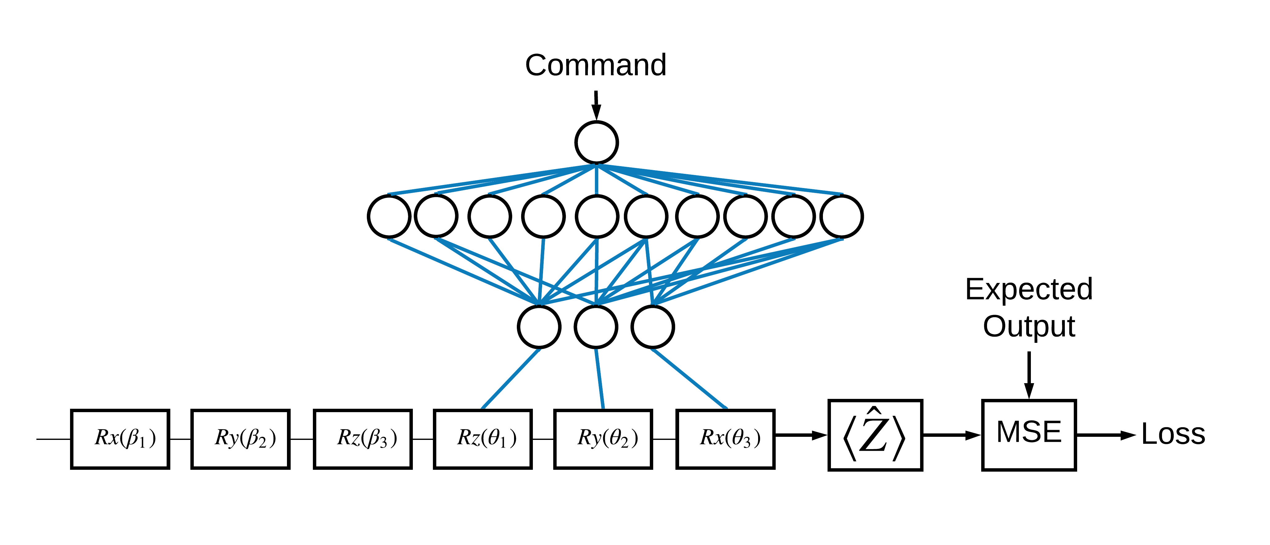
Now that you've seen the basics, let's use TensorFlow Quantum to construct a hybrid quantum-classical neural net. You will train a classical neural net to control a single qubit. The control will be optimized to correctly prepare the qubit in the 0 or 1 state, overcoming a simulated systematic calibration error. This figure shows the architecture:

Even without a neural network this is a straightforward problem to solve, but the theme is similar to the real quantum control problems you might solve using TFQ. It demonstrates an end-to-end example of a quantum-classical computation using the tfq.layers.ControlledPQC (Parametrized Quantum Circuit) layer inside of a tf.keras.Model.
For the implementation of this tutorial, this architecture is split into 3 parts:
- The input circuit or datapoint circuit: The first three \(R\) gates.
- The controlled circuit: The other three \(R\) gates.
- The controller: The classical neural-network setting the parameters of the controlled circuit.
2.1 The controlled circuit definition
Define a learnable single bit rotation, as indicated in the figure above. This will correspond to our controlled circuit.
# Parameters that the classical NN will feed values into.
control_params = sympy.symbols('theta_1 theta_2 theta_3')

# Create the parameterized circuit.
qubit = cirq.GridQubit(0, 0)
model_circuit = cirq.Circuit(
    cirq.rz(control_params[0])(qubit),
    cirq.ry(control_params[1])(qubit),
    cirq.rx(control_params[2])(qubit))

SVGCircuit(model_circuit)
findfont: Font family 'Arial' not found.
findfont: Font family 'Arial' not found.
findfont: Font family 'Arial' not found.
findfont: Font family 'Arial' not found.
2.2 The controller
Now define controller network:
# The classical neural network layers.
controller = tf.keras.Sequential(
    [tf.keras.layers.Dense(10, activation='elu'),
     tf.keras.layers.Dense(3)])
Given a batch of commands, the controller outputs a batch of control signals for the controlled circuit.
The controller is randomly initialized so these outputs are not useful, yet.
controller(tf.constant([[0.0], [1.0]])).numpy()
array([[ 0.        ,  0.        ,  0.        ],
       [-0.933574  ,  0.11334291,  0.2570168 ]], dtype=float32)
2.3 Connect the controller to the circuit
Use tfq to connect the controller to the controlled circuit, as a single keras.Model.
See the Keras Functional API guide for more about this style of model definition.
First define the inputs to the model:
# This input is the simulated miscalibration that the model will learn to correct.
circuits_input = tf.keras.Input(
    shape=(),
    # The circuit-tensor has dtype `tf.string`
    dtype=tf.string,
    name='circuits_input')

# Commands will be either `0` or `1`, specifying the state to set the qubit to.
commands_input = tf.keras.Input(shape=(1,),
                                dtype=tf.dtypes.float32,
                                name='commands_input')
Next apply operations to those inputs, to define the computation.
dense_2 = controller(commands_input)

# TFQ layer for classically controlled circuits.
expectation_layer = tfq.layers.ControlledPQC(
    model_circuit,
    # Observe Z
    operators=cirq.Z(qubit))
expectation = expectation_layer([circuits_input, dense_2])
Now package this computation as a tf.keras.Model:
# The full Keras model is built from our layers.
model = tf.keras.Model(inputs=[circuits_input, commands_input],
                       outputs=expectation)
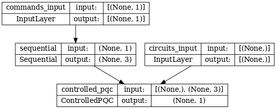
The network architecture is indicated by the plot of the model below. Compare this model plot to the architecture diagram to verify correctness.
tf.keras.utils.plot_model(model, show_shapes=True, dpi=70)

This model takes two inputs: The commands for the controller, and the input-circuit whose output the controller is attempting to correct.
2.4 The dataset
The model attempts to output the correct correct measurement value of \(\hat{Z}\) for each command. The commands and correct values are defined below.
# The command input values to the classical NN.
commands = np.array([[0], [1]], dtype=np.float32)

# The desired Z expectation value at output of quantum circuit.
expected_outputs = np.array([[1], [-1]], dtype=np.float32)
This is not the entire training dataset for this task. Each datapoint in the dataset also needs an input circuit.
2.4 Input circuit definition
The input-circuit below defines the random miscalibration the model will learn to correct.
random_rotations = np.random.uniform(0, 2 * np.pi, 3)
noisy_preparation = cirq.Circuit(
    cirq.rx(random_rotations[0])(qubit),
    cirq.ry(random_rotations[1])(qubit),
    cirq.rz(random_rotations[2])(qubit))
datapoint_circuits = tfq.convert_to_tensor([noisy_preparation] *
                                           2)  # Make two copied of this circuit
There are two copies of the circuit, one for each datapoint.
datapoint_circuits.shape
TensorShape([2])
2.5 Training
With the inputs defined you can test-run the tfq model.
model([datapoint_circuits, commands]).numpy()
array([[0.9958177 ],
       [0.98207647]], dtype=float32)
Now run a standard training process to adjust these values towards the expected_outputs.
optimizer = tf.keras.optimizers.Adam(learning_rate=0.05)
loss = tf.keras.losses.MeanSquaredError()
model.compile(optimizer=optimizer, loss=loss)
history = model.fit(x=[datapoint_circuits, commands],
                    y=expected_outputs,
                    epochs=30,
                    verbose=0)
plt.plot(history.history['loss'])
plt.title("Learning to Control a Qubit")
plt.xlabel("Iterations")
plt.ylabel("Error in Control")
plt.show()

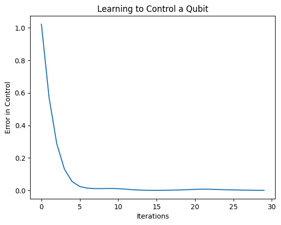
From this plot you can see that the neural network has learned to overcome the systematic miscalibration.
2.6 Verify outputs
Now use the trained model, to correct the qubit calibration errors. With Cirq:
def check_error(command_values, desired_values):
    """Based on the value in `command_value` see how well you could prepare
  the full circuit to have `desired_value` when taking expectation w.r.t. Z."""
    params_to_prepare_output = controller(command_values).numpy()
    full_circuit = noisy_preparation + model_circuit

    # Test how well you can prepare a state to get expectation the expectation
    # value in `desired_values`
    for index in [0, 1]:
        state = cirq_simulator.simulate(full_circuit, {
            s: v
            for (s, v) in zip(control_params, params_to_prepare_output[index])
        }).final_state_vector
        expt = cirq.Z(qubit).expectation_from_state_vector(state, {
            qubit: 0
        }).real
        print(
            f'For a desired output (expectation) of {desired_values[index]} with'
            f' noisy preparation, the controller\nnetwork found the following '
            f'values for theta: {params_to_prepare_output[index]}\nWhich gives an'
            f' actual expectation of: {expt}\n')


check_error(commands, expected_outputs)
For a desired output (expectation) of [1.] with noisy preparation, the controller
network found the following values for theta: [-0.12697363  0.2161613  -0.43002388]
Which gives an actual expectation of: 0.8917269706726074

For a desired output (expectation) of [-1.] with noisy preparation, the controller
network found the following values for theta: [-0.39836413  0.28400192  3.2667234 ]
Which gives an actual expectation of: -0.9761434197425842
The value of the loss function during training provides a rough idea of how well the model is learning. The lower the loss, the closer the expectation values in the above cell is to desired_values. If you aren't as concerned with the parameter values, you can always check the outputs from above using tfq:
model([datapoint_circuits, commands])
<tf.Tensor: shape=(2, 1), dtype=float32, numpy=
array([[ 0.8917272],
       [-0.9761431]], dtype=float32)>
3 Learning to prepare eigenstates of different operators
The choice of the \(\pm \hat{Z}\) eigenstates corresponding to 1 and 0 was arbitrary. You could have just as easily wanted 1 to correspond to the \(+ \hat{Z}\) eigenstate and 0 to correspond to the \(-\hat{X}\) eigenstate. One way to accomplish this is by specifying a different measurement operator for each command, as indicated in the figure below:

This requires use of tfq.layers.Expectation. Now your input has grown to include three objects: circuit, command, and operator. The output is still the expectation value.
3.1 New model definition
Lets take a look at the model to accomplish this task:
# Define inputs.
commands_input = tf.keras.layers.Input(shape=(1),
                                       dtype=tf.dtypes.float32,
                                       name='commands_input')
circuits_input = tf.keras.Input(
    shape=(),
    # The circuit-tensor has dtype `tf.string`
    dtype=tf.dtypes.string,
    name='circuits_input')
operators_input = tf.keras.Input(shape=(1,),
                                 dtype=tf.dtypes.string,
                                 name='operators_input')
Here is the controller network:
# Define classical NN.
controller = tf.keras.Sequential(
    [tf.keras.layers.Dense(10, activation='elu'),
     tf.keras.layers.Dense(3)])
Combine the circuit and the controller into a single keras.Model using tfq:
dense_2 = controller(commands_input)

# Since you aren't using a PQC or ControlledPQC you must append
# your model circuit onto the datapoint circuit tensor manually.
full_circuit = tfq.layers.AddCircuit()(circuits_input, append=model_circuit)
expectation_output = tfq.layers.Expectation()(full_circuit,
                                              symbol_names=control_params,
                                              symbol_values=dense_2,
                                              operators=operators_input)

# Contruct your Keras model.
two_axis_control_model = tf.keras.Model(
    inputs=[circuits_input, commands_input, operators_input],
    outputs=[expectation_output])
3.2 The dataset
Now you will also include the operators you wish to measure for each datapoint you supply for model_circuit:
# The operators to measure, for each command.
operator_data = tfq.convert_to_tensor([[cirq.X(qubit)], [cirq.Z(qubit)]])

# The command input values to the classical NN.
commands = np.array([[0], [1]], dtype=np.float32)

# The desired expectation value at output of quantum circuit.
expected_outputs = np.array([[1], [-1]], dtype=np.float32)
3.3 Training
Now that you have your new inputs and outputs you can train once again using keras.
optimizer = tf.keras.optimizers.Adam(learning_rate=0.05)
loss = tf.keras.losses.MeanSquaredError()

two_axis_control_model.compile(optimizer=optimizer, loss=loss)

history = two_axis_control_model.fit(
    x=[datapoint_circuits, commands, operator_data],
    y=expected_outputs,
    epochs=30,
    verbose=1)
Epoch 1/30
1/1 [==============================] - 0s 448ms/step - loss: 2.1220
Epoch 2/30
1/1 [==============================] - 0s 4ms/step - loss: 1.1681
Epoch 3/30
1/1 [==============================] - 0s 4ms/step - loss: 0.4768
Epoch 4/30
1/1 [==============================] - 0s 4ms/step - loss: 0.2370
Epoch 5/30
1/1 [==============================] - 0s 4ms/step - loss: 0.1323
Epoch 6/30
1/1 [==============================] - 0s 4ms/step - loss: 0.1373
Epoch 7/30
1/1 [==============================] - 0s 4ms/step - loss: 0.2637
Epoch 8/30
1/1 [==============================] - 0s 4ms/step - loss: 0.3070
Epoch 9/30
1/1 [==============================] - 0s 4ms/step - loss: 0.2497
Epoch 10/30
1/1 [==============================] - 0s 4ms/step - loss: 0.1425
Epoch 11/30
1/1 [==============================] - 0s 4ms/step - loss: 0.0502
Epoch 12/30
1/1 [==============================] - 0s 4ms/step - loss: 0.0089
Epoch 13/30
1/1 [==============================] - 0s 4ms/step - loss: 6.0734e-04
Epoch 14/30
1/1 [==============================] - 0s 4ms/step - loss: 1.4278e-04
Epoch 15/30
1/1 [==============================] - 0s 4ms/step - loss: 5.3596e-04
Epoch 16/30
1/1 [==============================] - 0s 4ms/step - loss: 0.0045
Epoch 17/30
1/1 [==============================] - 0s 4ms/step - loss: 0.0149
Epoch 18/30
1/1 [==============================] - 0s 4ms/step - loss: 0.0298
Epoch 19/30
1/1 [==============================] - 0s 4ms/step - loss: 0.0435
Epoch 20/30
1/1 [==============================] - 0s 4ms/step - loss: 0.0502
Epoch 21/30
1/1 [==============================] - 0s 4ms/step - loss: 0.0482
Epoch 22/30
1/1 [==============================] - 0s 4ms/step - loss: 0.0395
Epoch 23/30
1/1 [==============================] - 0s 4ms/step - loss: 0.0283
Epoch 24/30
1/1 [==============================] - 0s 4ms/step - loss: 0.0183
Epoch 25/30
1/1 [==============================] - 0s 4ms/step - loss: 0.0115
Epoch 26/30
1/1 [==============================] - 0s 4ms/step - loss: 0.0080
Epoch 27/30
1/1 [==============================] - 0s 4ms/step - loss: 0.0067
Epoch 28/30
1/1 [==============================] - 0s 4ms/step - loss: 0.0064
Epoch 29/30
1/1 [==============================] - 0s 4ms/step - loss: 0.0063
Epoch 30/30
1/1 [==============================] - 0s 4ms/step - loss: 0.0059
plt.plot(history.history['loss'])
plt.title("Learning to Control a Qubit")
plt.xlabel("Iterations")
plt.ylabel("Error in Control")
plt.show()

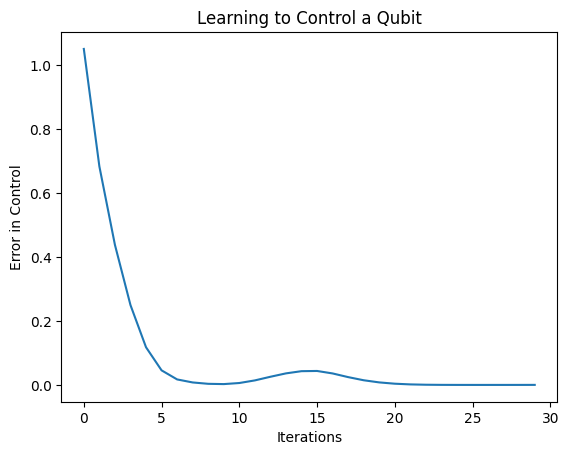
The loss function has dropped to zero.
The controller is available as a stand-alone model. Call the controller, and check its response to each command signal. It would take some work to correctly compare these outputs to the contents of random_rotations.
controller.predict(np.array([0, 1]))
1/1 [==============================] - 0s 61ms/step
array([[1.6359813 , 2.0209079 , 0.9253092 ],
       [4.635884  , 0.11778158, 3.192774  ]], dtype=float32)
