 View on TensorFlow.org View on TensorFlow.org
|
 Run in Google Colab Run in Google Colab
|
 View source on GitHub View source on GitHub
|
 Download notebook Download notebook
|
Building off of the comparisons made in the MNIST tutorial, this tutorial explores the recent work of Huang et al. that shows how different datasets affect performance comparisons. In the work, the authors seek to understand how and when classical machine learning models can learn as well as (or better than) quantum models. The work also showcases an empirical performance separation between classical and quantum machine learning model via a carefully crafted dataset. You will:
- Prepare a reduced dimension Fashion-MNIST dataset.
- Use quantum circuits to re-label the dataset and compute Projected Quantum Kernel features (PQK).
- Train a classical neural network on the re-labeled dataset and compare the performance with a model that has access to the PQK features.
Setup
Install TensorFlow and TensorFlow Quantum:
# In Colab, you will be asked to restart the session after this finishes.pip install tensorflow==2.18.1 tensorflow-quantum==0.7.6
Configure the use of Keras 2:
import os

# Keras 2 must be selected before importing TensorFlow or TensorFlow Quantum:
os.environ["TF_USE_LEGACY_KERAS"] = "1"
Now import TensorFlow, TensorFlow Quantum, and other modules needed:
import cirq
import sympy
import numpy as np
import tensorflow as tf
import tensorflow_quantum as tfq

# visualization tools
%matplotlib inline
import matplotlib.pyplot as plt
from cirq.contrib.svg import SVGCircuit
np.random.seed(1234)
1. Data preparation
You will begin by preparing the fashion-MNIST dataset for running on a quantum computer.
1.1 Download fashion-MNIST
The first step is to get the traditional fashion-mnist dataset. This can be done using the tf.keras.datasets module.
(x_train, y_train), (x_test,
                     y_test) = tf.keras.datasets.fashion_mnist.load_data()

# Rescale the images from [0,255] to the [0.0,1.0] range.
x_train, x_test = x_train / 255.0, x_test / 255.0

print("Number of original training examples:", len(x_train))
print("Number of original test examples:", len(x_test))
Number of original training examples: 60000
Number of original test examples: 10000
Filter the dataset to keep just the T-shirts/tops and dresses, remove the other classes. At the same time convert the label, y, to boolean: True for 0 and False for 3.
def filter_03(x, y):
    keep = (y == 0) | (y == 3)
    x, y = x[keep], y[keep]
    y = y == 0
    return x, y
x_train, y_train = filter_03(x_train, y_train)
x_test, y_test = filter_03(x_test, y_test)

print("Number of filtered training examples:", len(x_train))
print("Number of filtered test examples:", len(x_test))
Number of filtered training examples: 12000
Number of filtered test examples: 2000
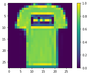
print(y_train[0])

plt.imshow(x_train[0, :, :])
plt.colorbar()
True
<matplotlib.colorbar.Colorbar at 0x7f6db42c3460>

1.2 Downscale the images
Just like the MNIST example, you will need to downscale these images in order to be within the boundaries for current quantum computers. This time however you will use a PCA transformation to reduce the dimensions instead of a tf.image.resize operation.
def truncate_x(x_train, x_test, n_components=10):
    """Perform PCA on image dataset keeping the top `n_components` components."""
    n_points_train = tf.gather(tf.shape(x_train), 0)
    n_points_test = tf.gather(tf.shape(x_test), 0)

    # Flatten to 1D
    x_train = tf.reshape(x_train, [n_points_train, -1])
    x_test = tf.reshape(x_test, [n_points_test, -1])

    # Normalize.
    feature_mean = tf.reduce_mean(x_train, axis=0)
    x_train_normalized = x_train - feature_mean
    x_test_normalized = x_test - feature_mean

    # Truncate.
    e_values, e_vectors = tf.linalg.eigh(
        tf.einsum('ji,jk->ik', x_train_normalized, x_train_normalized))
    return tf.einsum('ij,jk->ik', x_train_normalized, e_vectors[:,-n_components:]), \
      tf.einsum('ij,jk->ik', x_test_normalized, e_vectors[:, -n_components:])
DATASET_DIM = 10
x_train, x_test = truncate_x(x_train, x_test, n_components=DATASET_DIM)
print(f'New datapoint dimension:', len(x_train[0]))
New datapoint dimension: 10
The last step is to reduce the size of the dataset to just 1000 training datapoints and 200 testing datapoints.
N_TRAIN = 1000
N_TEST = 200
x_train, x_test = x_train[:N_TRAIN], x_test[:N_TEST]
y_train, y_test = y_train[:N_TRAIN], y_test[:N_TEST]
print("New number of training examples:", len(x_train))
print("New number of test examples:", len(x_test))
New number of training examples: 1000
New number of test examples: 200
2. Relabeling and computing PQK features
You will now prepare a "stilted" quantum dataset by incorporating quantum components and re-labeling the truncated fashion-MNIST dataset you've created above. In order to get the most seperation between quantum and classical methods, you will first prepare the PQK features and then relabel outputs based on their values.
2.1 Quantum encoding and PQK features
You will create a new set of features, based on x_train, y_train, x_test and y_test that is defined to be the 1-RDM on all qubits of:
\(V(x_{\text{train} } / n_{\text{trotter} }) ^ {n_{\text{trotter} } } U_{\text{1qb} } | 0 \rangle\)
Where \(U_\text{1qb}\) is a wall of single qubit rotations and \(V(\hat{\theta}) = e^{-i\sum_i \hat{\theta_i} (X_i X_{i+1} + Y_i Y_{i+1} + Z_i Z_{i+1})}\)
First, you can generate the wall of single qubit rotations:
def single_qubit_wall(qubits, rotations):
    """Prepare a single qubit X,Y,Z rotation wall on `qubits`."""
    wall_circuit = cirq.Circuit()
    for i, qubit in enumerate(qubits):
        for j, gate in enumerate([cirq.X, cirq.Y, cirq.Z]):
            wall_circuit.append(gate(qubit)**rotations[i][j])

    return wall_circuit
You can quickly verify this works by looking at the circuit:
SVGCircuit(
    single_qubit_wall(cirq.GridQubit.rect(1, 4),
                      np.random.uniform(size=(4, 3))))
Next you can prepare \(V(\hat{\theta})\) with the help of tfq.util.exponential which can exponentiate any commuting cirq.PauliSum objects:
def v_theta(qubits):
    """Prepares a circuit that generates V(\theta)."""
    ref_paulis = [
        cirq.X(q0) * cirq.X(q1) + \
        cirq.Y(q0) * cirq.Y(q1) + \
        cirq.Z(q0) * cirq.Z(q1) for q0, q1 in zip(qubits, qubits[1:])
    ]
    exp_symbols = list(sympy.symbols('ref_0:' + str(len(ref_paulis))))
    return tfq.util.exponential(ref_paulis, exp_symbols), exp_symbols
This circuit might be a little bit harder to verify by looking at, but you can still examine a two qubit case to see what is happening:
test_circuit, test_symbols = v_theta(cirq.GridQubit.rect(1, 2))
print(f'Symbols found in circuit:{test_symbols}')
SVGCircuit(test_circuit)
Symbols found in circuit:[ref_0]
Now you have all the building blocks you need to put your full encoding circuits together:
def prepare_pqk_circuits(qubits, classical_source, n_trotter=10):
    """Prepare the pqk feature circuits around a dataset."""
    n_qubits = len(qubits)
    n_points = len(classical_source)

    # Prepare random single qubit rotation wall.
    random_rots = np.random.uniform(-2, 2, size=(n_qubits, 3))
    initial_U = single_qubit_wall(qubits, random_rots)

    # Prepare parametrized V
    V_circuit, symbols = v_theta(qubits)
    exp_circuit = cirq.Circuit(V_circuit for t in range(n_trotter))

    # Convert to `tf.Tensor`
    initial_U_tensor = tfq.convert_to_tensor([initial_U])
    initial_U_splat = tf.tile(initial_U_tensor, [n_points])

    full_circuits = tfq.layers.AddCircuit()(initial_U_splat, append=exp_circuit)
    # Replace placeholders in circuits with values from `classical_source`.
    return tfq.resolve_parameters(
        full_circuits, tf.convert_to_tensor([str(x) for x in symbols]),
        tf.convert_to_tensor(classical_source * (n_qubits / 3) / n_trotter))
Choose some qubits and prepare the data encoding circuits:
qubits = cirq.GridQubit.rect(1, DATASET_DIM + 1)
q_x_train_circuits = prepare_pqk_circuits(qubits, x_train)
q_x_test_circuits = prepare_pqk_circuits(qubits, x_test)
Next, compute the PQK features based on the 1-RDM of the dataset circuits above and store the results in rdm, a tf.Tensor with shape [n_points, n_qubits, 3]. The entries in rdm[i][j][k] = \(\langle \psi_i | OP^k_j | \psi_i \rangle\) where i indexes over datapoints, j indexes over qubits and k indexes over \(\lbrace \hat{X}, \hat{Y}, \hat{Z} \rbrace\) .
def get_pqk_features(qubits, data_batch):
    """Get PQK features based on above construction."""
    ops = [[cirq.X(q), cirq.Y(q), cirq.Z(q)] for q in qubits]
    ops_tensor = tf.expand_dims(tf.reshape(tfq.convert_to_tensor(ops), -1), 0)
    batch_dim = tf.gather(tf.shape(data_batch), 0)
    ops_splat = tf.tile(ops_tensor, [batch_dim, 1])
    exp_vals = tfq.layers.Expectation()(data_batch, operators=ops_splat)
    rdm = tf.reshape(exp_vals, [batch_dim, len(qubits), -1])
    return rdm
x_train_pqk = get_pqk_features(qubits, q_x_train_circuits)
x_test_pqk = get_pqk_features(qubits, q_x_test_circuits)
print('New PQK training dataset has shape:', x_train_pqk.shape)
print('New PQK testing dataset has shape:', x_test_pqk.shape)
New PQK training dataset has shape: (1000, 11, 3)
New PQK testing dataset has shape: (200, 11, 3)
2.2 Re-labeling based on PQK features
Now that you have these quantum generated features in x_train_pqk and x_test_pqk, it is time to re-label the dataset. To achieve maximum seperation between quantum and classical performance you can re-label the dataset based on the spectrum information found in x_train_pqk and x_test_pqk.
def compute_kernel_matrix(vecs, gamma):
    """Computes d[i][j] = e^ -gamma * (vecs[i] - vecs[j]) ** 2 """
    scaled_gamma = gamma / (tf.cast(tf.gather(tf.shape(vecs), 1), tf.float32) *
                            tf.math.reduce_std(vecs))
    return scaled_gamma * tf.einsum('ijk->ij', (vecs[:, None, :] - vecs)**2)


def get_spectrum(datapoints, gamma=1.0):
    """Compute the eigenvalues and eigenvectors of the kernel of datapoints."""
    KC_qs = compute_kernel_matrix(datapoints, gamma)
    S, V = tf.linalg.eigh(KC_qs)
    S = tf.math.abs(S)
    return S, V
S_pqk, V_pqk = get_spectrum(
    tf.reshape(tf.concat([x_train_pqk, x_test_pqk], 0),
               [-1, len(qubits) * 3]))

S_original, V_original = get_spectrum(tf.cast(tf.concat([x_train, x_test], 0),
                                              tf.float32),
                                      gamma=0.005)

print('Eigenvectors of pqk kernel matrix:', V_pqk)
print('Eigenvectors of original kernel matrix:', V_original)
Eigenvectors of pqk kernel matrix: tf.Tensor(
[[-2.09569391e-02  1.05973557e-02  2.16634180e-02 ...  2.80352887e-02
   1.55521873e-02  2.82677952e-02]
 [-2.29303762e-02  4.66355234e-02  7.91163836e-03 ... -6.14174758e-04
  -7.07804322e-01  2.85902526e-02]
 [-1.77853629e-02 -3.00758495e-03 -2.55225878e-02 ... -2.40783971e-02
   2.11018627e-03  2.69009806e-02]
 ...
 [ 6.05797209e-02  1.32483775e-02  2.69536003e-02 ... -1.38843581e-02
   3.05043962e-02  3.85345481e-02]
 [ 6.33309558e-02 -3.04112374e-03  9.77444276e-03 ...  7.48321265e-02
   3.42793856e-03  3.67484428e-02]
 [ 5.86028099e-02  5.84433973e-03  2.64811981e-03 ...  2.82612257e-02
  -3.80136147e-02  3.29943895e-02]], shape=(1200, 1200), dtype=float32)
Eigenvectors of original kernel matrix: tf.Tensor(
[[ 0.03835681  0.0283473  -0.01169789 ...  0.02343717  0.0211248
   0.03206972]
 [-0.04018159  0.00888097 -0.01388255 ...  0.00582427  0.717551
   0.02881948]
 [-0.0166719   0.01350376 -0.03663862 ...  0.02467175 -0.00415936
   0.02195409]
 ...
 [-0.03015648 -0.01671632 -0.01603392 ...  0.00100583 -0.00261221
   0.02365689]
 [ 0.0039777  -0.04998879 -0.00528336 ...  0.01560401 -0.04330755
   0.02782002]
 [-0.01665728 -0.00818616 -0.0432341  ...  0.00088256  0.00927396
   0.01875088]], shape=(1200, 1200), dtype=float32)
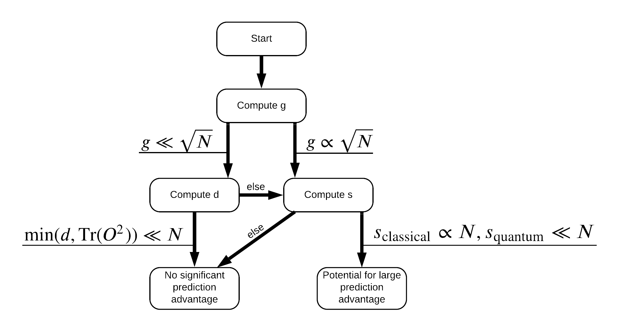
Now you have everything you need to re-label the dataset! Now you can consult with the flowchart to better understand how to maximize performance seperation when re-labeling the dataset:

In order to maximize the seperation between quantum and classical models, you will attempt to maximize the geometric difference between the original dataset and the PQK features kernel matrices \(g(K_1 || K_2) = \sqrt{ || \sqrt{K_2} K_1^{-1} \sqrt{K_2} || _\infty}\) using S_pqk, V_pqk and S_original, V_original. A large value of \(g\) ensures that you initially move to the right in the flowchart down towards a prediction advantage in the quantum case.
def get_stilted_dataset(S, V, S_2, V_2, lambdav=1.1):
    """Prepare new labels that maximize geometric distance between kernels."""
    S_diag = tf.linalg.diag(S**0.5)
    S_2_diag = tf.linalg.diag(S_2 / (S_2 + lambdav)**2)
    scaling = S_diag @ tf.transpose(V) @ \
              V_2 @ S_2_diag @ tf.transpose(V_2) @ \
              V @ S_diag

    # Generate new lables using the largest eigenvector.
    _, vecs = tf.linalg.eig(scaling)
    new_labels = tf.math.real(
        tf.einsum('ij,j->i', tf.cast(V @ S_diag, tf.complex64),
                  vecs[-1])).numpy()
    # Create new labels and add some small amount of noise.
    final_y = new_labels > np.median(new_labels)
    noisy_y = (final_y ^ (np.random.uniform(size=final_y.shape) > 0.95))
    return noisy_y
y_relabel = get_stilted_dataset(S_pqk, V_pqk, S_original, V_original)
y_train_new, y_test_new = y_relabel[:N_TRAIN], y_relabel[N_TRAIN:]
3. Comparing models
Now that you have prepared your dataset it is time to compare model performance. You will create two small feedforward neural networks and compare performance when they are given access to the PQK features found in x_train_pqk.
3.1 Create PQK enhanced model
Using standard tf.keras library features you can now create and a train a model on the x_train_pqk and y_train_new datapoints:
#docs_infra: no_execute
def create_pqk_model():
    model = tf.keras.Sequential()
    model.add(
        tf.keras.layers.Dense(32,
                              activation='sigmoid',
                              input_shape=[
                                  len(qubits) * 3,
                              ]))
    model.add(tf.keras.layers.Dense(16, activation='sigmoid'))
    model.add(tf.keras.layers.Dense(1))
    return model


pqk_model = create_pqk_model()
pqk_model.compile(loss=tf.keras.losses.BinaryCrossentropy(from_logits=True),
                  optimizer=tf.keras.optimizers.Adam(learning_rate=0.003),
                  metrics=['accuracy'])

pqk_model.summary()
Model: "sequential"
_________________________________________________________________
Layer (type)                 Output Shape              Param #
=================================================================
dense (Dense)                (None, 32)                1088
_________________________________________________________________
dense_1 (Dense)              (None, 16)                528
_________________________________________________________________
dense_2 (Dense)              (None, 1)                 17
=================================================================
Total params: 1,633
Trainable params: 1,633
Non-trainable params: 0
_________________________________________________________________
#docs_infra: no_execute
pqk_history = pqk_model.fit(tf.reshape(x_train_pqk, [N_TRAIN, -1]),
                            y_train_new,
                            batch_size=32,
                            epochs=1000,
                            verbose=0,
                            validation_data=(tf.reshape(x_test_pqk,
                                                        [N_TEST, -1]),
                                             y_test_new))
3.2 Create a classical model
Similar to the code above you can now also create a classical model that doesn't have access to the PQK features in your stilted dataset. This model can be trained using x_train and y_label_new.
#docs_infra: no_execute
def create_fair_classical_model():
    model = tf.keras.Sequential()
    model.add(
        tf.keras.layers.Dense(32,
                              activation='sigmoid',
                              input_shape=[
                                  DATASET_DIM,
                              ]))
    model.add(tf.keras.layers.Dense(16, activation='sigmoid'))
    model.add(tf.keras.layers.Dense(1))
    return model


model = create_fair_classical_model()
model.compile(loss=tf.keras.losses.BinaryCrossentropy(from_logits=True),
              optimizer=tf.keras.optimizers.Adam(learning_rate=0.03),
              metrics=['accuracy'])

model.summary()
Model: "sequential_1"
_________________________________________________________________
Layer (type)                 Output Shape              Param #
=================================================================
dense_3 (Dense)              (None, 32)                352
_________________________________________________________________
dense_4 (Dense)              (None, 16)                528
_________________________________________________________________
dense_5 (Dense)              (None, 1)                 17
=================================================================
Total params: 897
Trainable params: 897
Non-trainable params: 0
_________________________________________________________________
#docs_infra: no_execute
classical_history = model.fit(x_train,
                              y_train_new,
                              batch_size=32,
                              epochs=1000,
                              verbose=0,
                              validation_data=(x_test, y_test_new))
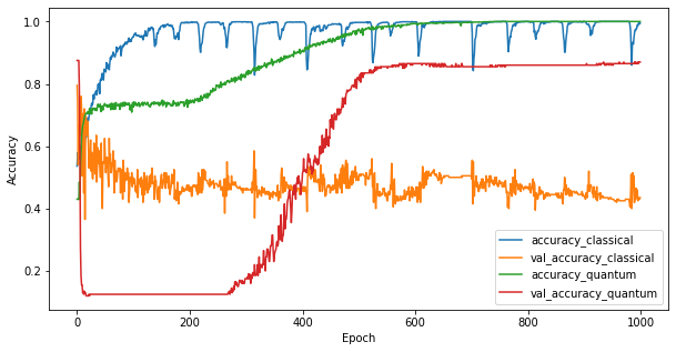
3.3 Compare performance
Now that you have trained the two models you can quickly plot the performance gaps in the validation data between the two. Typically both models will achieve > 0.9 accuaracy on the training data. However on the validation data it becomes clear that only the information found in the PQK features is enough to make the model generalize well to unseen instances.
#docs_infra: no_execute
plt.figure(figsize=(10, 5))
plt.plot(classical_history.history['accuracy'], label='accuracy_classical')
plt.plot(classical_history.history['val_accuracy'],
         label='val_accuracy_classical')
plt.plot(pqk_history.history['accuracy'], label='accuracy_quantum')
plt.plot(pqk_history.history['val_accuracy'], label='val_accuracy_quantum')
plt.xlabel('Epoch')
plt.ylabel('Accuracy')
plt.legend()
<matplotlib.legend.Legend at 0x7f6d846ecee0>

4. Important conclusions
There are several important conclusions you can draw from this and the MNIST experiments:
It's very unlikely that the quantum models of today will beat classical model performance on classical data. Especially on today's classical datasets that can have upwards of a million datapoints.
Just because the data might come from a hard to classically simulate quantum circuit, doesn't necessarily make the data hard to learn for a classical model.
Datasets (ultimately quantum in nature) that are easy for quantum models to learn and hard for classical models to learn do exist, regardless of model architecture or training algorithms used.
