
| |
|
 在 GitHub 上查看源代码 在 GitHub 上查看源代码
|
|
简介
此笔记本使用 TensorFlow Core 低级 API 展示了 TensorFlow 作为高性能科学计算平台的能力。访问 Core API 概述以详细了解 TensorFlow Core 及其预期用例。
本教程探讨奇异值分解 (SVD) 技术及其在低秩逼近问题中的应用。SVD 用于分解实数或复数矩阵,并在数据科学中具有多种用例,例如图像压缩。本教程的图像来自 Google Brain 的 Imagen 项目。
安装
import matplotlib
from matplotlib.image import imread
from matplotlib import pyplot as plt
import requests
# Preset Matplotlib figure sizes.
matplotlib.rcParams['figure.figsize'] = [16, 9]
import tensorflow as tf
print(tf.__version__)
2022-12-14 22:07:37.487775: W tensorflow/compiler/xla/stream_executor/platform/default/dso_loader.cc:64] Could not load dynamic library 'libnvinfer.so.7'; dlerror: libnvinfer.so.7: cannot open shared object file: No such file or directory
2022-12-14 22:07:37.487870: W tensorflow/compiler/xla/stream_executor/platform/default/dso_loader.cc:64] Could not load dynamic library 'libnvinfer_plugin.so.7'; dlerror: libnvinfer_plugin.so.7: cannot open shared object file: No such file or directory
2022-12-14 22:07:37.487879: W tensorflow/compiler/tf2tensorrt/utils/py_utils.cc:38] TF-TRT Warning: Cannot dlopen some TensorRT libraries. If you would like to use Nvidia GPU with TensorRT, please make sure the missing libraries mentioned above are installed properly.
2.11.0
SVD 基础知识
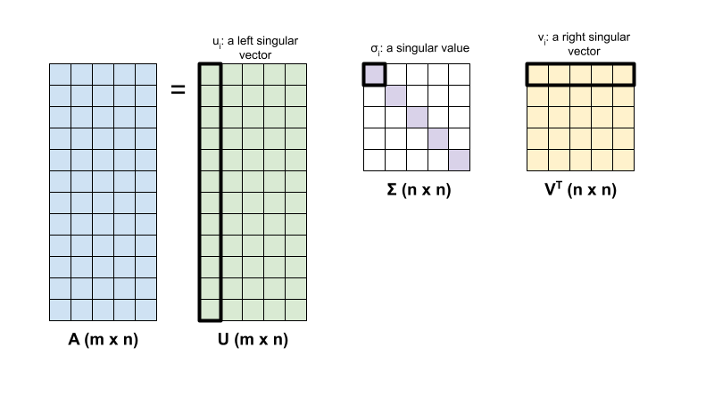
矩阵 \({\mathrm{A} }\) 的奇异值分解由以下因式分解确定:
\[{\mathrm{A} } = {\mathrm{U} } \Sigma {\mathrm{V} }^T\]
其中
- \(\underset{m \times n}{\mathrm{A} }\):输入矩阵,其中 \(m \geq n\)
- \(\underset{m \times n}{\mathrm{U} }\):正交矩阵,\({\mathrm{U} }^T{\mathrm{U} } = {\mathrm{I} }\),包含各个列 \(u_i\),表示 \({\mathrm{A} }\) 的左奇异向量
- \(\underset{n \times n}{\Sigma}\):对角矩阵,包含各个对角条目 \(\sigma_i\),表示\({\mathrm{A} }\)的奇异值
- \(\underset{n \times n}{ {\mathrm{V} }^T}\):正交矩阵,\({\mathrm{V} }^T{\mathrm{V} } = {\mathrm{I} }\),包含各个行 \(v_i\),表示 \({\mathrm{A} }\) 的右奇异向量
当 \(m < n\) 时,\({\mathrm{U} }\) 和 \(\Sigma\) 的维度均为 \((m \times m)\),而 \({\mathrm{V} }^T\) 的维度为 \((m \times n)\)。
TensorFlow 的线性代数软件包具有一个函数 tf.linalg.svd,可用于计算一个或多个矩阵的奇异值分解。首先,定义一个简单的矩阵并计算其 SVD 因式分解。
A = tf.random.uniform(shape=[40,30])
# Compute the SVD factorization
s, U, V = tf.linalg.svd(A)
# Define Sigma and V Transpose
S = tf.linalg.diag(s)
V_T = tf.transpose(V)
# Reconstruct the original matrix
A_svd = U@S@V_T
# Visualize
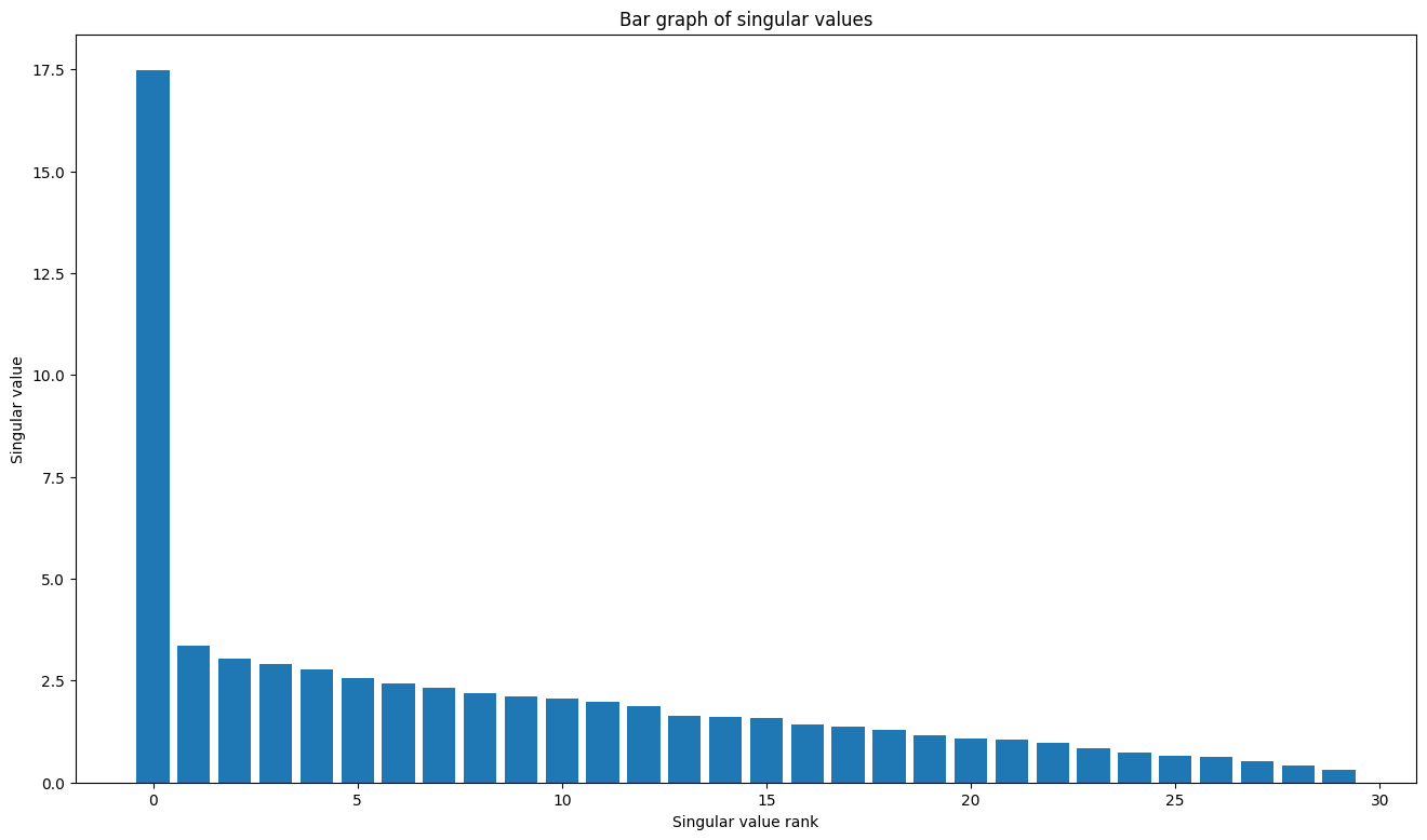
plt.bar(range(len(s)), s);
plt.xlabel("Singular value rank")
plt.ylabel("Singular value")
plt.title("Bar graph of singular values");
tf.einsum 函数可用于根据 tf.linalg.svd 的输出直接计算矩阵重构。
A_svd = tf.einsum('s,us,vs -> uv',s,U,V)
print('\nReconstructed Matrix, A_svd', A_svd)
Reconstructed Matrix, A_svd tf.Tensor(
[[0.08873153 0.8545857  0.17131968 ... 0.75293845 0.5527939  0.47924733]
 [0.700058   0.19823846 0.82784504 ... 0.8284904  0.39280835 0.55723095]
 [0.2696367  0.8009648  0.20029528 ... 0.01831989 0.4325177  0.51484114]
 ...
 [0.03570056 0.29680276 0.67311686 ... 0.35031977 0.68188447 0.56625783]
 [0.27047342 0.29453754 0.41465694 ... 0.576772   0.31444252 0.23378772]
 [0.92036074 0.75892895 0.35073748 ... 0.9658414  0.5708384  0.63662905]], shape=(40, 30), dtype=float32)
使用 SVD 进行低秩逼近
矩阵的秩 \({\mathrm{A} }\) 由其各列所跨越的向量空间的维度决定。SVD 可用于逼近具有较低秩的矩阵,这最终会降低存储矩阵表示的信息所需数据的维数。
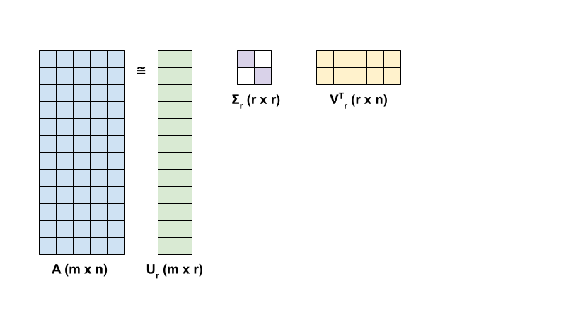
\({\mathrm{A} }\) 在 SVD 中的秩 r 逼近由以下方程定义:
\[{\mathrm{A_r} } = {\mathrm{U_r} } \Sigma_r {\mathrm{V_r} }^T\]
其中
- \(\underset{m \times r}{\mathrm{U_r} }\):由 \({\mathrm{U} }\) 的前 \(r\) 列组成的矩阵
- \(\underset{r \times r}{\Sigma_r}\):由\(\Sigma\) 中的前 \(r\) 个奇异值组成的对角矩阵
- \(\underset{r \times n}{\mathrm{V_r} }^T\):由 \({\mathrm{V} }^T\) 的前 \(r\) 行组成的矩阵
首先,编写一个函数来计算给定矩阵的秩 r 逼近。这种低秩逼近过程用于图像压缩;因此,计算每个逼近的物理数据大小也很有帮助。为简单起见,假设秩 r 逼近矩阵的数据大小等于计算逼近所需的元素总数。接下来,编写一个函数来呈现原始矩阵 \(\mathrm{A}\)、其秩 r 逼近 \(\mathrm{A}_r\) 和误差矩阵 \(|\mathrm{A} - \mathrm{A}_r|\)。
def rank_r_approx(s, U, V, r, verbose=False):
  # Compute the matrices necessary for a rank-r approximation
  s_r, U_r, V_r = s[..., :r], U[..., :, :r], V[..., :, :r] # ... implies any number of extra batch axes
  # Compute the low-rank approximation and its size
  A_r = tf.einsum('...s,...us,...vs->...uv',s_r,U_r,V_r)
  A_r_size = tf.size(U_r) + tf.size(s_r) + tf.size(V_r)
  if verbose:
    print(f"Approximation Size: {A_r_size}")
  return A_r, A_r_size

def viz_approx(A, A_r):
  # Plot A, A_r, and A - A_r
  vmin, vmax = 0, tf.reduce_max(A)
  fig, ax = plt.subplots(1,3)
  mats = [A, A_r, abs(A - A_r)]
  titles = ['Original A', 'Approximated A_r', 'Error |A - A_r|']
  for i, (mat, title) in enumerate(zip(mats, titles)):
    ax[i].pcolormesh(mat, vmin=vmin, vmax=vmax)
    ax[i].set_title(title)
    ax[i].axis('off')
print(f"Original Size of A: {tf.size(A)}")
s, U, V = tf.linalg.svd(A)
Original Size of A: 1200
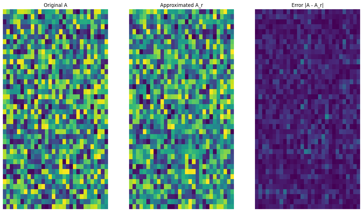
# Rank-15 approximation
A_15, A_15_size = rank_r_approx(s, U, V, 15, verbose = True)
viz_approx(A, A_15)
Approximation Size: 1065
# Rank-3 approximation
A_3, A_3_size = rank_r_approx(s, U, V, 3, verbose = True)
viz_approx(A, A_3)
Approximation Size: 213
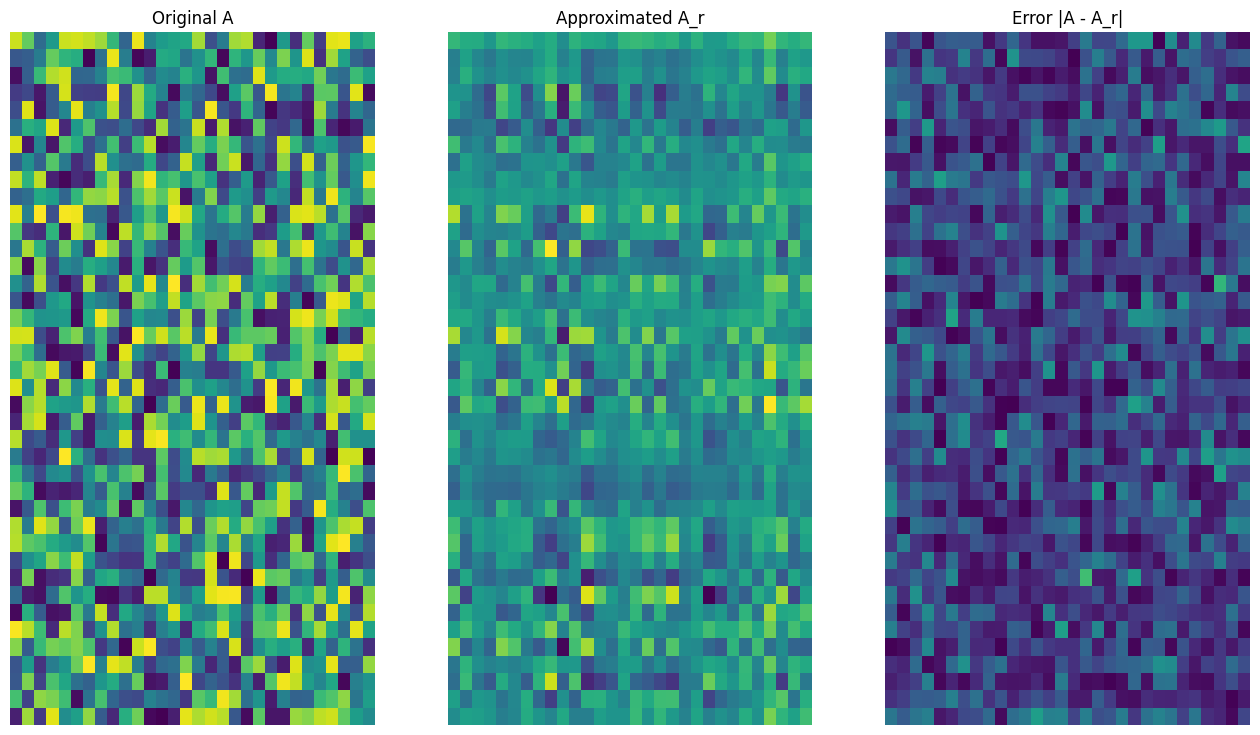
正如预期的那样,使用较低的秩会得到不太准确的逼近。然而,这些低秩逼近的质量在现实世界的场景中通常足够好。另请注意,使用 SVD 进行低秩逼近的主要目标是减少数据的维数,而不是减少数据本身的磁盘空间。不过,随着输入矩阵的维度变高,许多低秩逼近也最终受益于缩减的数据大小。这种缩减的好处是该过程适用于图像压缩问题的原因。
图像加载
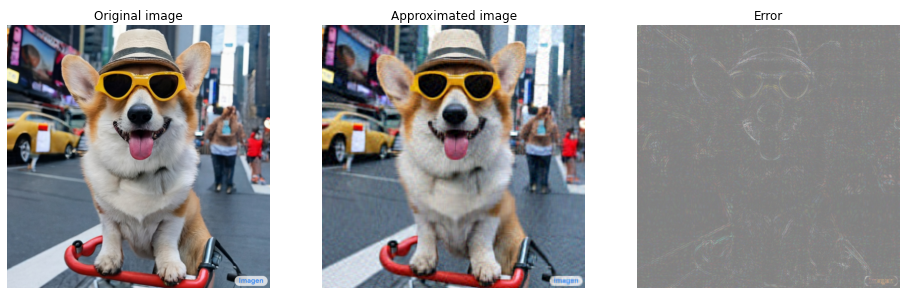
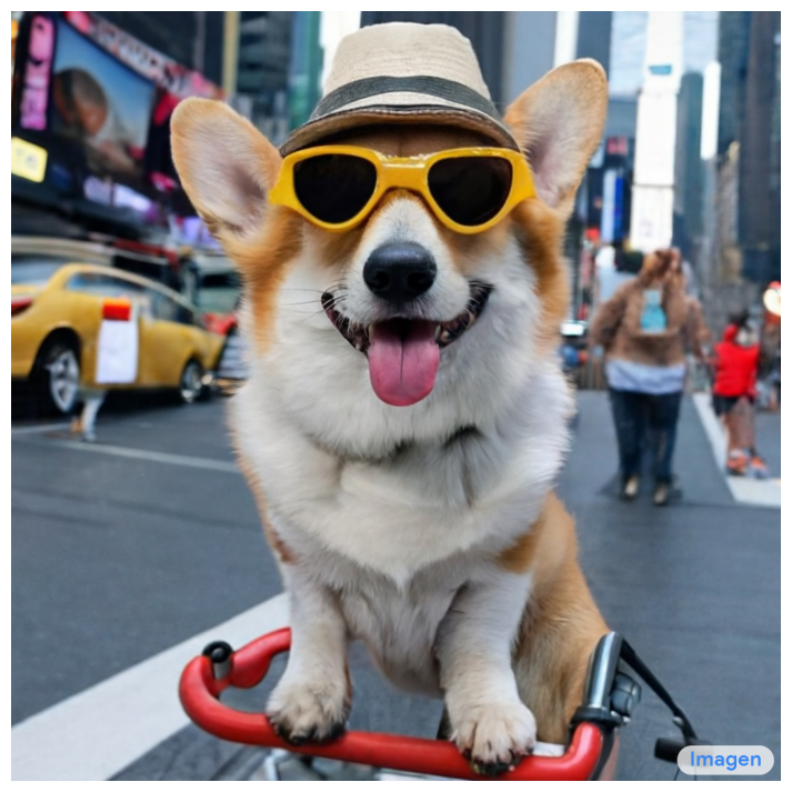
Imagen 首页上提供了以下图像。Imagen 是由 Google Research 的 Brain 团队开发的文本到图像扩散模型。AI 根据提示创建了这张图像:“一张柯基犬在时代广场骑自行车的照片。它戴着墨镜和沙滩帽。”多么酷啊!您还可以将下面的网址更改为任何 .jpg 链接以加载选择的自定义图像。
首先,读入并呈现图像。读取 JPEG 文件后,Matplotlib 会输出一个形状为 \((m \times n \times 3)\) 的矩阵 \({\mathrm{I} }\),它表示一个二维图像,具有分别对应于红色、绿色和蓝色的 3 个颜色通道。
img_link = "https://imagen.research.google/main_gallery_images/a-photo-of-a-corgi-dog-riding-a-bike-in-times-square.jpg"
img_path = requests.get(img_link, stream=True).raw
I = imread(img_path, 0)
print("Input Image Shape:", I.shape)
Input Image Shape: (1024, 1024, 3)
def show_img(I):
  # Display the image in matplotlib
  img = plt.imshow(I)
  plt.axis('off')
  return
show_img(I)
图像压缩算法
现在,使用 SVD 计算样本图像的低秩逼近。回想一下,图像的形状为 \((1024 \times 1024 \times 3)\),并且 SVD 理论仅适用于二维矩阵。这意味着必须将样本图像批处理为 3 个大小相等的矩阵,这些矩阵对应于 3 个颜色通道中的每一个。这可以通过将矩阵转置为形状 \((3 \times 1024 \times 1024)\) 来实现。为了清楚地呈现逼近误差,将图像的 RGB 值从 \([0,255]\) 重新缩放到 \([0,1]\)。记得在呈现它们之前将逼近值裁剪到此区间内。tf.clip_by_value 函数对此十分有用。
def compress_image(I, r, verbose=False):
  # Compress an image with the SVD given a rank
  I_size = tf.size(I)
  print(f"Original size of image: {I_size}")
  # Compute SVD of image
  I = tf.convert_to_tensor(I)/255
  I_batched = tf.transpose(I, [2, 0, 1]) # einops.rearrange(I, 'h w c -> c h w')
  s, U, V = tf.linalg.svd(I_batched)
  # Compute low-rank approximation of image across each RGB channel
  I_r, I_r_size = rank_r_approx(s, U, V, r)
  I_r = tf.transpose(I_r, [1, 2, 0]) # einops.rearrange(I_r, 'c h w -> h w c')
  I_r_prop = (I_r_size / I_size)
  if verbose:
    # Display compressed image and attributes
    print(f"Number of singular values used in compression: {r}")
    print(f"Compressed image size: {I_r_size}")
    print(f"Proportion of original size: {I_r_prop:.3f}")
    ax_1 = plt.subplot(1,2,1)
    show_img(tf.clip_by_value(I_r,0.,1.))
    ax_1.set_title("Approximated image")
    ax_2 = plt.subplot(1,2,2)
    show_img(tf.clip_by_value(0.5+abs(I-I_r),0.,1.))
    ax_2.set_title("Error")
  return I_r, I_r_prop
现在,计算以下秩的秩 r 逼近:100、50、10
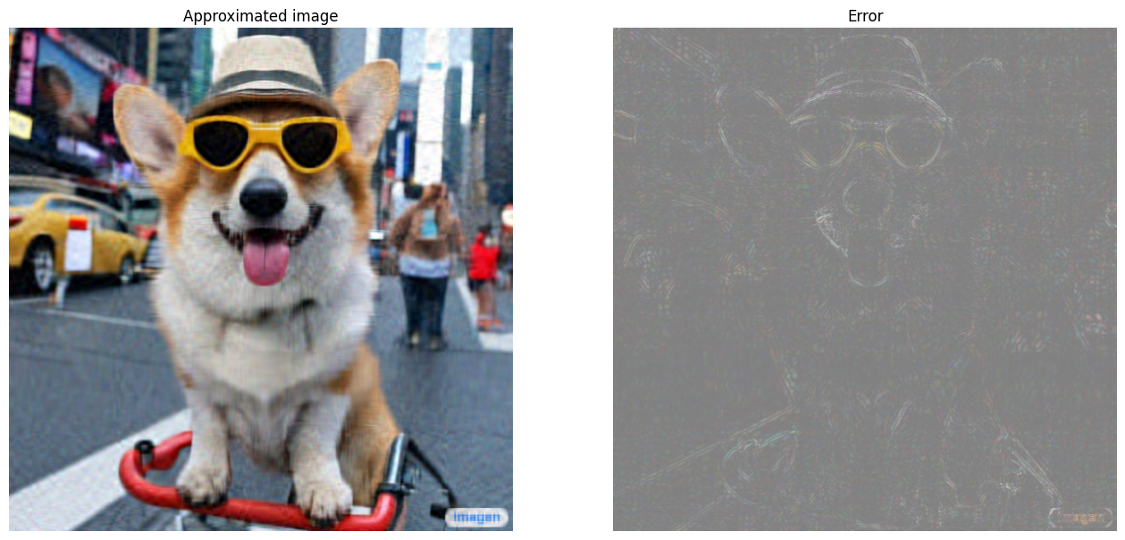
I_100, I_100_prop = compress_image(I, 100, verbose=True)
Original size of image: 3145728
Number of singular values used in compression: 100
Compressed image size: 614700
Proportion of original size: 0.195
I_50, I_50_prop = compress_image(I, 50, verbose=True)
Original size of image: 3145728
Number of singular values used in compression: 50
Compressed image size: 307350
Proportion of original size: 0.098
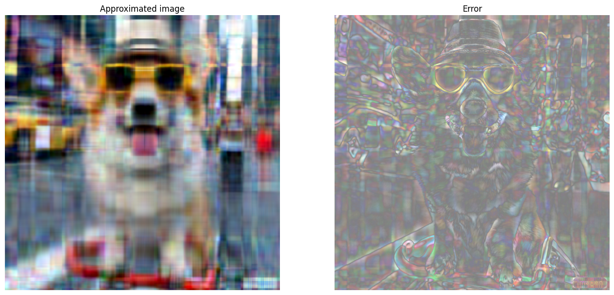
I_10, I_10_prop = compress_image(I, 10, verbose=True)
Original size of image: 3145728
Number of singular values used in compression: 10
Compressed image size: 61470
Proportion of original size: 0.020
评估逼近
可以通过多种有趣的方法衡量有效性并更好地控制矩阵逼近。
压缩因子与秩
对于上述每个逼近,观察数据大小如何随秩变化。
plt.figure(figsize=(11,6))
plt.plot([100, 50, 10], [I_100_prop, I_50_prop, I_10_prop])
plt.xlabel("Rank")
plt.ylabel("Proportion of original image size")
plt.title("Compression factor vs rank");
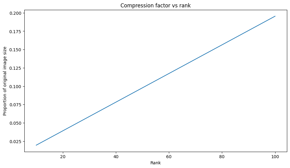
基于这张图,逼近图像的压缩因子与其秩之间存在线性关系。为了进一步探索这一点,回想一下,逼近矩阵 \({\mathrm{A} }_r\) 的数据大小被定义为其计算所需的元素总数。下面的方程可用于找出压缩因子与秩之间的关系:
\[x = (m \times r) + r + (r \times n) = r \times (m + n + 1)\]
\[c = \large \frac{x}{y} = \frac{r \times (m + n + 1)}{m \times n}\]
其中
- \(x\):\({\mathrm{A_r} }\) 的大小
- \(y\):\({\mathrm{A} }\) 的大小
- \(c = \frac{x}{y}\):压缩因子
- \(r\):逼近的秩
- \(m\) 和 \(n\):\({\mathrm{A} }\) 的行维度和列维度
为了找到将图像压缩到所需因子 \(c\) 所需的秩 \(r\),可以重新排列上述方程以求解 \(r\):
\[r = ⌊{\large\frac{c \times m \times n}{m + n + 1} }⌋\]
请注意,此公式与颜色通道维度无关,因为各个 RGB 逼近不会相互影响。现在,编写一个函数来压缩给定所需压缩因子的输入图像。
def compress_image_with_factor(I, compression_factor, verbose=False):
  # Returns a compressed image based on a desired compression factor
  m,n,o = I.shape
  r = int((compression_factor * m * n)/(m + n + 1))
  I_r, I_r_prop = compress_image(I, r, verbose=verbose)
  return I_r
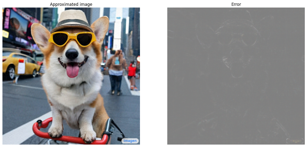
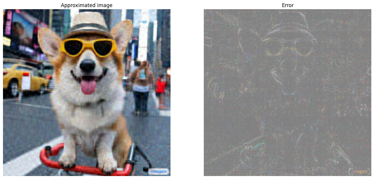
将图像压缩到其原始大小的 15%。
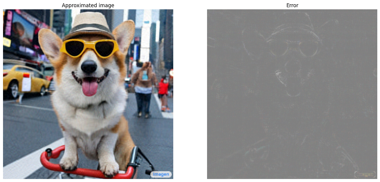
compression_factor = 0.15
I_r_img = compress_image_with_factor(I, compression_factor, verbose=True)
Original size of image: 3145728
Number of singular values used in compression: 76
Compressed image size: 467172
Proportion of original size: 0.149
奇异值的累积和
奇异值的累积总和可作为秩 r 逼近捕获的能量量的有用指标。呈现样本图像中奇异值的 RGB 平均累积比例。tf.cumsum 函数对此十分有用。
def viz_energy(I):
  # Visualize the energy captured based on rank
  # Computing SVD
  I = tf.convert_to_tensor(I)/255
  I_batched = tf.transpose(I, [2, 0, 1])
  s, U, V = tf.linalg.svd(I_batched)
  # Plotting average proportion across RGB channels
  props_rgb = tf.map_fn(lambda x: tf.cumsum(x)/tf.reduce_sum(x), s)
  props_rgb_mean = tf.reduce_mean(props_rgb, axis=0)
  plt.figure(figsize=(11,6))
  plt.plot(range(len(I)), props_rgb_mean, color='k')
  plt.xlabel("Rank / singular value number")
  plt.ylabel("Cumulative proportion of singular values")
  plt.title("RGB-averaged proportion of energy captured by the first 'r' singular values")
viz_energy(I)
WARNING:tensorflow:From /tmpfs/src/tf_docs_env/lib/python3.9/site-packages/tensorflow/python/autograph/pyct/static_analysis/liveness.py:83: Analyzer.lamba_check (from tensorflow.python.autograph.pyct.static_analysis.liveness) is deprecated and will be removed after 2023-09-23.
Instructions for updating:
Lambda fuctions will be no more assumed to be used in the statement where they are used, or at least in the same block. https://github.com/tensorflow/tensorflow/issues/56089
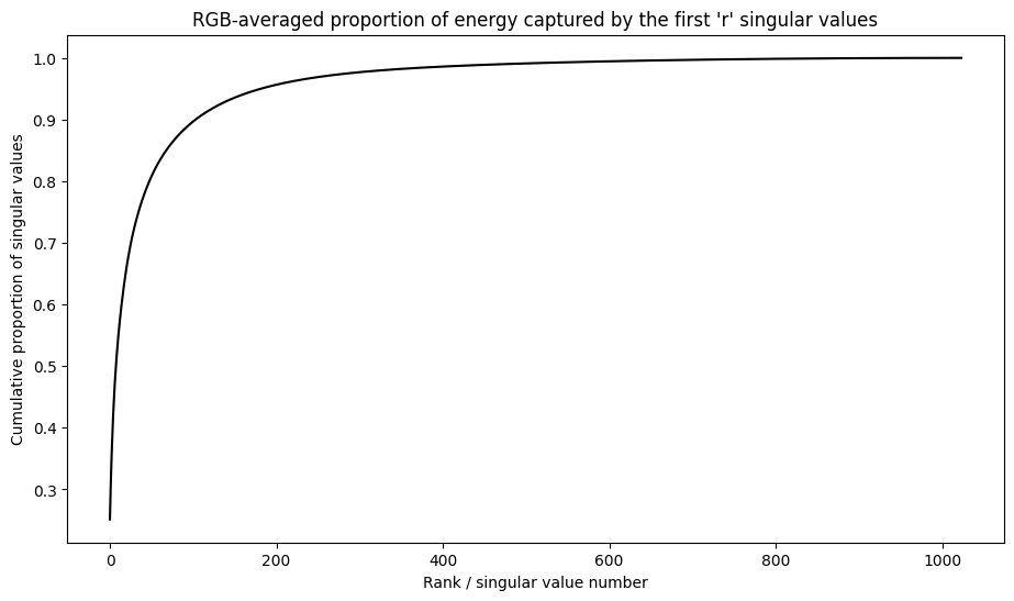
看起来这个图像中超过 90% 的能量是在前 100 个奇异值中捕获的。现在,编写一个函数来压缩给定所需能量保留因子的输入图像。
def compress_image_with_energy(I, energy_factor, verbose=False):
  # Returns a compressed image based on a desired energy factor
  # Computing SVD
  I_rescaled = tf.convert_to_tensor(I)/255
  I_batched = tf.transpose(I_rescaled, [2, 0, 1])
  s, U, V = tf.linalg.svd(I_batched)
  # Extracting singular values
  props_rgb = tf.map_fn(lambda x: tf.cumsum(x)/tf.reduce_sum(x), s)
  props_rgb_mean = tf.reduce_mean(props_rgb, axis=0)
  # Find closest r that corresponds to the energy factor
  r = tf.argmin(tf.abs(props_rgb_mean - energy_factor)) + 1
  actual_ef = props_rgb_mean[r]
  I_r, I_r_prop = compress_image(I, r, verbose=verbose)
  print(f"Proportion of energy captured by the first {r} singular values: {actual_ef:.3f}")
  return I_r
压缩图像以保留 75% 的能量。
energy_factor = 0.75
I_r_img = compress_image_with_energy(I, energy_factor, verbose=True)
Original size of image: 3145728
Number of singular values used in compression: 35
Compressed image size: 215145
Proportion of original size: 0.068
Proportion of energy captured by the first 35 singular values: 0.753
误差和奇异值
逼近误差与奇异值之间也存在一个有趣的关系。事实证明,逼近的平方 Frobenius 范数等于其被省略的奇异值的平方和:
\[{||A - A_r||}^2 = \sum_{i=r+1}^{R}σ_i^2\]
使用本教程开头的示例矩阵的秩 10 逼近来测试这种关系。
s, U, V = tf.linalg.svd(A)
A_10, A_10_size = rank_r_approx(s, U, V, 10)
squared_norm = tf.norm(A - A_10)**2
s_squared_sum = tf.reduce_sum(s[10:]**2)
print(f"Squared Frobenius norm: {squared_norm:.3f}")
print(f"Sum of squared singular values left out: {s_squared_sum:.3f}")
Squared Frobenius norm: 32.054
Sum of squared singular values left out: 32.054
结论
此笔记本介绍了使用 TensorFlow 实现奇异值分解并将其应用于编写图像压缩算法的过程。下面是一些可能有所帮助的提示:
- TensorFlow Core API 可用于各种高性能科学计算用例。
- 要详细了解 TensorFlow 线性代数功能,请访问 linalg 模块的文档。
- SVD 也可应用于构建推荐系统。
有关使用 TensorFlow Core API 的更多示例,请查阅指南。如果您想详细了解如何加载和准备数据,请参阅有关图像数据加载或 CSV 数据加载的教程。