TensorFlow Core API 快速入门

在 TensorFlow.org 上查看

在 Google Colab 中运行

在 Github 上查看源代码

下载笔记本

本快速入门教程演示了如何使用 TensorFlow Core 低级 API 来构建和训练预测燃油效率的多元线性回归模型。它使用 Auto MPG 数据集，其中包含 20 世纪 70 年代末和 20 世纪 80 年代初汽车的燃油效率数据。

您将遵循机器学习过程的典型阶段：

加载数据集。
构建输入流水线。
构建多元线性回归模型。
评估模型的性能。

安装

首先，导入 TensorFlow 和其他必要的库：

import tensorflow as tf
import pandas as pd
import matplotlib
from matplotlib import pyplot as plt
print("TensorFlow version:", tf.__version__)
# Set a random seed for reproducible results 
tf.random.set_seed(22)

2022-12-14 22:12:24.670018: W tensorflow/compiler/xla/stream_executor/platform/default/dso_loader.cc:64] Could not load dynamic library 'libnvinfer.so.7'; dlerror: libnvinfer.so.7: cannot open shared object file: No such file or directory
2022-12-14 22:12:24.670122: W tensorflow/compiler/xla/stream_executor/platform/default/dso_loader.cc:64] Could not load dynamic library 'libnvinfer_plugin.so.7'; dlerror: libnvinfer_plugin.so.7: cannot open shared object file: No such file or directory
2022-12-14 22:12:24.670133: W tensorflow/compiler/tf2tensorrt/utils/py_utils.cc:38] TF-TRT Warning: Cannot dlopen some TensorRT libraries. If you would like to use Nvidia GPU with TensorRT, please make sure the missing libraries mentioned above are installed properly.
TensorFlow version: 2.11.0

加载和预处理数据集

接下来，您需要从 UCI Machine Learning Repository 加载和预处理 Auto MPG 数据集。该数据集使用气缸、排量、马力和重量等各种定量和分类特征来预测 20 世纪 70 年代末和 20 世纪 80 年代初汽车的燃油效率。

数据集包含一些未知值。确保使用 pandas.DataFrame.dropna 去除任何缺失值，并使用 tf.convert_to_tensor 和 tf.cast 函数将数据集转换为 tf.float32 张量类型。

url = 'http://archive.ics.uci.edu/ml/machine-learning-databases/auto-mpg/auto-mpg.data'
column_names = ['MPG', 'Cylinders', 'Displacement', 'Horsepower', 'Weight',
                'Acceleration', 'Model Year', 'Origin']

dataset = pd.read_csv(url, names=column_names, na_values='?', comment='\t',
                          sep=' ', skipinitialspace=True)

dataset = dataset.dropna()
dataset_tf = tf.convert_to_tensor(dataset, dtype=tf.float32)
dataset.tail()

接下来，将数据集拆分为训练集和测试集。确保使用 tf.random.shuffle 重排数据集，以避免有偏差的拆分。

dataset_shuffled = tf.random.shuffle(dataset_tf, seed=22)
train_data, test_data = dataset_shuffled[100:], dataset_shuffled[:100]
x_train, y_train = train_data[:, 1:], train_data[:, 0]
x_test, y_test = test_data[:, 1:], test_data[:, 0]

通过对 "Origin" 特征进行独热编码来执行基本特征工程。tf.one_hot 函数可用于将此分类列转换为 3 个单独的二进制列。

def onehot_origin(x):
  origin = tf.cast(x[:, -1], tf.int32)
  # Use `origin - 1` to account for 1-indexed feature
  origin_oh = tf.one_hot(origin - 1, 3)
  x_ohe = tf.concat([x[:, :-1], origin_oh], axis = 1)
  return x_ohe

x_train_ohe, x_test_ohe = onehot_origin(x_train), onehot_origin(x_test)
x_train_ohe.numpy()

array([[  4., 140.,  72., ...,   1.,   0.,   0.],
       [  4., 120.,  74., ...,   0.,   0.,   1.],
       [  4., 122.,  88., ...,   0.,   1.,   0.],
       ...,
       [  8., 318., 150., ...,   1.,   0.,   0.],
       [  4., 156., 105., ...,   1.,   0.,   0.],
       [  6., 232., 100., ...,   1.,   0.,   0.]], dtype=float32)

此示例显示了一个多元回归问题，其中预测器或特征具有截然不同的尺度。因此，标准化数据以使每个特征具有零均值和单位方差会有所帮助。使用 tf.reduce_mean 和 tf.math.reduce_std 函数进行标准化。然后，可以对回归模型的预测进行非标准化以获得其用原始单位表示的值。

class Normalize(tf.Module):
  def __init__(self, x):
    # Initialize the mean and standard deviation for normalization
    self.mean = tf.math.reduce_mean(x, axis=0)
    self.std = tf.math.reduce_std(x, axis=0)

  def norm(self, x):
    # Normalize the input
    return (x - self.mean)/self.std

  def unnorm(self, x):
    # Unnormalize the input
    return (x * self.std) + self.mean

norm_x = Normalize(x_train_ohe)
norm_y = Normalize(y_train)
x_train_norm, y_train_norm = norm_x.norm(x_train_ohe), norm_y.norm(y_train)
x_test_norm, y_test_norm = norm_x.norm(x_test_ohe), norm_y.norm(y_test)

构建机器学习模型

使用 TensorFlow Core API 构建线性回归模型。多元线性回归的方程如下：

\[{\mathrm{Y} } = {\mathrm{X} }w + b\]

其中

\(\underset{m\times 1}{\mathrm{Y} }\)：目标向量
\(\underset{m\times n}{\mathrm{X} }\)：特征矩阵
\(\underset{n\times 1}w\)：权重向量
\(b\)：偏差

通过使用 @tf.function 装饰器，跟踪相应的 Python 代码以生成可调用的 TensorFlow 计算图。这种方式有利于在训练后保存和加载模型。它还可以为具有多层和复杂运算的模型带来性能提升。

class LinearRegression(tf.Module):

  def __init__(self):
    self.built = False

  @tf.function
  def __call__(self, x):
    # Initialize the model parameters on the first call
    if not self.built:
      # Randomly generate the weight vector and bias term
      rand_w = tf.random.uniform(shape=[x.shape[-1], 1])
      rand_b = tf.random.uniform(shape=[])
      self.w = tf.Variable(rand_w)
      self.b = tf.Variable(rand_b)
      self.built = True
    y = tf.add(tf.matmul(x, self.w), self.b)
    return tf.squeeze(y, axis=1)

对于每个样本，该模型通过计算其特征的加权和加上一个偏差项来返回对输入汽车 MPG 的预测值。然后，可以对该预测值进行非标准化以获得其用原始单位表示的值。

lin_reg = LinearRegression()
prediction = lin_reg(x_train_norm[:1])
prediction_unnorm = norm_y.unnorm(prediction)
prediction_unnorm.numpy()

array([6.8007374], dtype=float32)

定义损失函数

现在，定义一个损失函数来评估模型在训练过程中的性能。

由于回归问题处理的是连续输出，均方误差 (MSE) 是损失函数的理想选择。MSE 由以下方程定义：

\[MSE = \frac{1}{m}\sum_{i=1}^{m}(\hat{y}_i -y_i)^2\]

其中

\(\hat{y}\)：预测向量
\(y\)：真实目标向量

此回归问题的目标是找到最小化 MSE 损失函数的最优权重向量 \(w\) 和偏差 \(b\)。

def mse_loss(y_pred, y):
  return tf.reduce_mean(tf.square(y_pred - y))

训练并评估模型

使用 mini-batch 进行训练既可以提高内存效率，又能加快收敛速度。tf.data.Dataset API 具有用于批处理和重排的有用函数。借助该 API，您可以从简单、可重用的部分构建复杂的输入流水线。在此指南中详细了解如何构建 TensorFlow 输入流水线。

batch_size = 64
train_dataset = tf.data.Dataset.from_tensor_slices((x_train_norm, y_train_norm))
train_dataset = train_dataset.shuffle(buffer_size=x_train.shape[0]).batch(batch_size)
test_dataset = tf.data.Dataset.from_tensor_slices((x_test_norm, y_test_norm))
test_dataset = test_dataset.shuffle(buffer_size=x_test.shape[0]).batch(batch_size)

接下来，编写一个训练循环，通过使用 MSE 损失函数及其相对于输入参数的梯度来迭代更新模型的参数。

这种迭代方法称为梯度下降。在每次迭代中，模型的参数通过在其计算梯度的相反方向上迈出一步来更新。这一步的大小由学习率决定，学习率是一个可配置的超参数。回想一下，函数的梯度表示其最陡上升的方向；因此，向相反方向迈出一步表示最陡下降的方向，这最终有助于最小化 MSE 损失函数。

# Set training parameters
epochs = 100
learning_rate = 0.01
train_losses, test_losses = [], []

# Format training loop
for epoch in range(epochs):
  batch_losses_train, batch_losses_test = [], []

  # Iterate through the training data
  for x_batch, y_batch in train_dataset:
    with tf.GradientTape() as tape:
      y_pred_batch = lin_reg(x_batch)
      batch_loss = mse_loss(y_pred_batch, y_batch)
    # Update parameters with respect to the gradient calculations
    grads = tape.gradient(batch_loss, lin_reg.variables)
    for g,v in zip(grads, lin_reg.variables):
      v.assign_sub(learning_rate * g)
    # Keep track of batch-level training performance 
    batch_losses_train.append(batch_loss)

  # Iterate through the testing data
  for x_batch, y_batch in test_dataset:
    y_pred_batch = lin_reg(x_batch)
    batch_loss = mse_loss(y_pred_batch, y_batch)
    # Keep track of batch-level testing performance 
    batch_losses_test.append(batch_loss)

  # Keep track of epoch-level model performance
  train_loss = tf.reduce_mean(batch_losses_train)
  test_loss = tf.reduce_mean(batch_losses_test)
  train_losses.append(train_loss)
  test_losses.append(test_loss)
  if epoch % 10 == 0:
    print(f'Mean squared error for step {epoch}: {train_loss.numpy():0.3f}')

# Output final losses
print(f"\nFinal train loss: {train_loss:0.3f}")
print(f"Final test loss: {test_loss:0.3f}")

Mean squared error for step 0: 2.866
Mean squared error for step 10: 0.453
Mean squared error for step 20: 0.285
Mean squared error for step 30: 0.231
Mean squared error for step 40: 0.209
Mean squared error for step 50: 0.203
Mean squared error for step 60: 0.194
Mean squared error for step 70: 0.184
Mean squared error for step 80: 0.186
Mean squared error for step 90: 0.176

Final train loss: 0.177
Final test loss: 0.157

绘制 MSE 损失随时间变化的图。计算指定验证集或测试集上的性能指标可确保模型不会对训练数据集过拟合，并且可以很好地泛化到未知数据。

matplotlib.rcParams['figure.figsize'] = [9, 6]

plt.plot(range(epochs), train_losses, label = "Training loss")
plt.plot(range(epochs), test_losses, label = "Testing loss")
plt.xlabel("Epoch")
plt.ylabel("Mean squared error loss")
plt.legend()
plt.title("MSE loss vs training iterations");

png

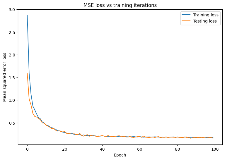
看起来该模型在拟合训练数据方面做得很好，同时也良好地泛化了未知测试数据。

保存和加载模型

首先，构建一个接受原始数据并执行以下运算的导出模块：

特征提取
归一化
预测
非归一化

class ExportModule(tf.Module):
  def __init__(self, model, extract_features, norm_x, norm_y):
    # Initialize pre and postprocessing functions
    self.model = model
    self.extract_features = extract_features
    self.norm_x = norm_x
    self.norm_y = norm_y

  @tf.function(input_signature=[tf.TensorSpec(shape=[None, None], dtype=tf.float32)]) 
  def __call__(self, x):
    # Run the ExportModule for new data points
    x = self.extract_features(x)
    x = self.norm_x.norm(x)
    y = self.model(x)
    y = self.norm_y.unnorm(y)
    return y

lin_reg_export = ExportModule(model=lin_reg,
                              extract_features=onehot_origin,
                              norm_x=norm_x,
                              norm_y=norm_y)

如果要将模型保存为当前状态，请使用 tf.saved_model.save 函数。要加载保存的模型并进行预测，请使用 tf.saved_model.load 函数。

import tempfile
import os

models = tempfile.mkdtemp()
save_path = os.path.join(models, 'lin_reg_export')
tf.saved_model.save(lin_reg_export, save_path)

INFO:tensorflow:Assets written to: /tmpfs/tmp/tmpu42sjkv0/lin_reg_export/assets

lin_reg_loaded = tf.saved_model.load(save_path)
test_preds = lin_reg_loaded(x_test)
test_preds[:10].numpy()

array([28.097498, 26.193336, 33.564373, 27.719315, 31.787924, 24.014559,
       24.421043, 13.45958 , 28.562454, 27.368694], dtype=float32)

结论

恭喜！您已经使用 TensorFlow Core 低级 API 训练了一个回归模型。

有关使用 TensorFlow Core API 的更多示例，请查看以下指南：

二元分类的逻辑回归
用于手写数字识别的多层感知器