阶乘混合

在此笔记本中，我们将展示如何使用 TensorFlow Probability (TFP) 从高斯分布的阶乘混合中进行采样，该阶乘混合定义为：\(p(x_1, ..., x_n) = \prod_i p_i(x_i)\) where: \(\begin{align*} p_i &\equiv \frac{1}{K}\sum_{i=1}^K \pi_{ik},\text{Normal}\left(\text{loc}=\mu_{ik},, \text{scale}=\sigma_{ik}\right)\1&=\sum_{k=1}^K\pi_{ik}, \forall i.\hphantom{MMMMMMMMMMM}\end{align*}\)

每个变量 \(x_i\) 都被建模为一个高斯混合，所有 \(n\) 变量的联合分布都是这些密度的乘积。

给定一个数据集 \(x^{(1)}, ..., x^{(T)}\)，我们将每个数据点 \(x^{(j)}\) 建模为一个高斯阶乘混合：\(p(x^{(j)}) = \prod_i p_i (x_i^{(j)})\)

阶乘混合是一种使用少量参数和大量模式创建分布的简单方式。

import tensorflow as tf
import numpy as np
import tensorflow_probability as tfp
import matplotlib.pyplot as plt
import seaborn as sns
tfd = tfp.distributions

# Use try/except so we can easily re-execute the whole notebook.
try:
  tf.enable_eager_execution()
except:
  pass

使用 TFP 构建高斯阶乘混合

num_vars = 2        # Number of variables (`n` in formula).
var_dim = 1         # Dimensionality of each variable `x[i]`.
num_components = 3  # Number of components for each mixture (`K` in formula).
sigma = 5e-2        # Fixed standard deviation of each component.

# Choose some random (component) modes.
component_mean = tfd.Uniform().sample([num_vars, num_components, var_dim])

factorial_mog = tfd.Independent(
   tfd.MixtureSameFamily(
       # Assume uniform weight on each component.
       mixture_distribution=tfd.Categorical(
           logits=tf.zeros([num_vars, num_components])),
       components_distribution=tfd.MultivariateNormalDiag(
           loc=component_mean, scale_diag=[sigma])),
   reinterpreted_batch_ndims=1)

请注意我们对 tfd.Independent 的使用。此“元分布”在 log_prob 计算中对最右边的 reinterpreted_batch_ndims 批次维度应用了 reduce_sum。在我们的示例中，这会在我们计算 log_prob 时加总变量维度，仅保留批次维度。请注意，这不会影响采样。

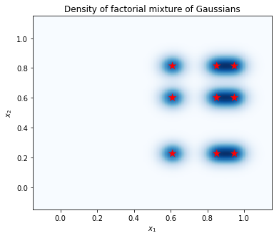
绘制密度

计算点网格上的密度，并用红星显示模式的位置。阶乘混合中的每个模式对应于底层高斯单变量混合的一对模式。我们可以在下面的图表中看到 9 个模式，但我们只需要 6 个参数（3 个用于在 \(x_1\) 中指定模式的位置，3 个用于在 \(x_2\) 中指定模式的位置）。相比之下，二维空间 \((x_1, x_2)\) 中的高斯混合分布需要 2 * 9 = 18 个参数来指定 9 个模式。

plt.figure(figsize=(6,5))

# Compute density.
nx = 250 # Number of bins per dimension.
x = np.linspace(-3 * sigma, 1 + 3 * sigma, nx).astype('float32')
vals = tf.reshape(tf.stack(np.meshgrid(x, x), axis=2), (-1, num_vars, var_dim))
probs = factorial_mog.prob(vals).numpy().reshape(nx, nx)

# Display as image.
from matplotlib.colors import ListedColormap
cmap = ListedColormap(sns.color_palette("Blues", 256))
p = plt.pcolor(x, x, probs, cmap=cmap)
ax = plt.axis('tight');

# Plot locations of means.
means_np = component_mean.numpy().squeeze()
for mu_x in means_np[0]:
  for mu_y in means_np[1]:
    plt.scatter(mu_x, mu_y, s=150, marker='*', c='r', edgecolor='none');
plt.axis(ax);

plt.xlabel('$x_1$')
plt.ylabel('$x_2$')
plt.title('Density of factorial mixture of Gaussians');

png

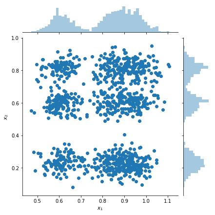
绘制样本和边缘密度估计

samples = factorial_mog.sample(1000).numpy()

g = sns.jointplot(
    x=samples[:, 0, 0],
    y=samples[:, 1, 0],
    kind="scatter",
    marginal_kws=dict(bins=50))
g.set_axis_labels("$x_1$", "$x_2$");

png