
| |
 在 Github 上查看源代码 在 Github 上查看源代码 |
|
TensorFlow Probability (TFP) 是用于进行概率推理和统计分析的库,现在也可以在 JAX 上运行!对于不熟悉 JAX 的人来说,JAX 是用于根据可组合的函数转换来加快数值计算的库。
JAX 上的 TFP 支持常规 TFP 中大量极为有用的功能,同时还保留了许多 TFP 用户现在习惯使用的抽象和 API。
设置
JAX 上的 TFP 不依赖于 TensorFlow;我们将 TensorFlow 从本 Colab 中完全卸载!
pip uninstall tensorflow -y -q我们可以使用最新的 Nightly 版本 TFP 在 JAX 上安装 TFP。
pip install -Uq tfp-nightly[jax] > /dev/null我们导入一些有用的 Python 库。
import matplotlib.pyplot as plt
import numpy as np
import seaborn as sns
from sklearn import datasets
sns.set(style='white')
/usr/local/lib/python3.6/dist-packages/statsmodels/tools/_testing.py:19: FutureWarning: pandas.util.testing is deprecated. Use the functions in the public API at pandas.testing instead.
  import pandas.util.testing as tm
我们再导入一些基本的 JAX 功能。
import jax.numpy as jnp
from jax import grad
from jax import jit
from jax import random
from jax import value_and_grad
from jax import vmap
在 JAX 上导入 TFP
要在 JAX 上使用 TFP,只需导入 jax“基质”,并像平常使用 tfp 那样使用该“基质”:
from tensorflow_probability.substrates import jax as tfp
tfd = tfp.distributions
tfb = tfp.bijectors
tfpk = tfp.math.psd_kernels
演示:贝叶斯逻辑回归
为了演示 JAX 后端的功能,我们将实现应用于经典 Iris 数据集的贝叶斯逻辑回归。
首先,导入 Iris 数据集,并提取一些元数据。
iris = datasets.load_iris()
features, labels = iris['data'], iris['target']

num_features = features.shape[-1]
num_classes = len(iris.target_names)
我们可以使用 tfd.JointDistributionCoroutine 定义该模型。我们将标准正态先验应用于权重和偏项,然后编写一个 target_log_prob 函数,用于将抽样标签固定到数据。
Root = tfd.JointDistributionCoroutine.Root
def model():
  w = yield Root(tfd.Sample(tfd.Normal(0., 1.),
                            sample_shape=(num_features, num_classes)))
  b = yield Root(
      tfd.Sample(tfd.Normal(0., 1.), sample_shape=(num_classes,)))
  logits = jnp.dot(features, w) + b
  yield tfd.Independent(tfd.Categorical(logits=logits),
                        reinterpreted_batch_ndims=1)


dist = tfd.JointDistributionCoroutine(model)
def target_log_prob(*params):
  return dist.log_prob(params + (labels,))
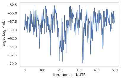
我们从 dist 中抽样,为 MCMC 生成初始状态。然后,我们可以定义一个函数,用于接受随机密钥和初始状态,并基于 No-U-Turn-Sampler (NUTS) 生成 500 个样本。请注意,我们可以使用 jit 等 JAX 转换通过 XLA 对 NUTS 抽样器进行编译。
init_key, sample_key = random.split(random.PRNGKey(0))
init_params = tuple(dist.sample(seed=init_key)[:-1])

@jit
def run_chain(key, state):
  kernel = tfp.mcmc.NoUTurnSampler(target_log_prob, 1e-3)
  return tfp.mcmc.sample_chain(500,
      current_state=state,
      kernel=kernel,
      trace_fn=lambda _, results: results.target_log_prob,
      num_burnin_steps=500,
      seed=key)

states, log_probs = run_chain(sample_key, init_params)
plt.figure()
plt.plot(log_probs)
plt.ylabel('Target Log Prob')
plt.xlabel('Iterations of NUTS')
plt.show()
我们使用我们的样本对每一组权重的预测概率求平均值,从而执行贝叶斯模型平均 (BMA)。
首先,我们编写一个函数,对于一组给定的参数,该函数将生成每个类的概率。我们可以使用 dist.sample_distributions 来获得模型中的最终分布。
def classifier_probs(params):
  dists, _ = dist.sample_distributions(seed=random.PRNGKey(0),
                                       value=params + (None,))
  return dists[-1].distribution.probs_parameter()
我们可以对这组样本执行 vmap(classifier_probs),从而获得每个样本的预测类概率。之后,我们计算每个样本的平均准确率,以及贝叶斯模型平均的准确率。
all_probs = jit(vmap(classifier_probs))(states)
print('Average accuracy:', jnp.mean(all_probs.argmax(axis=-1) == labels))
print('BMA accuracy:', jnp.mean(all_probs.mean(axis=0).argmax(axis=-1) == labels))
Average accuracy: 0.96952
BMA accuracy: 0.97999996
BMA 似乎可以将我们的错误率减少差不多三分之一!
基本原理
JAX 上的 TFP 与 TF 具有相同的 API,它接受 JAX 模拟量,而不是 tf.Tensor 等 TF 对象。例如,在 tf.Tensor 以前用作输入的位置,该 API 现在应该使用 JAX DeviceArray。TFP 方法将返回 DeviceArray,而不是 tf.Tensor。JAX 上的 TFP 也使用 JAX 对象的嵌套结构,例如 DeviceArray 列表或字典。
分布
TFP 的大多数分布都可以在 JAX 中使用,其语义与 TF 对应项极为类似。这些分布也作为 JAX Pytree 注册,因此可以作为 JAX 转换函数的输入和输出。
基本分布
分布的 log_prob 方法运行方式相同。
dist = tfd.Normal(0., 1.)
print(dist.log_prob(0.))
-0.9189385
从分布中抽样时,需要明确传入 PRNGKey(或一组整数)作为 seed 关键字参数。如果无法明确传入种子,将会引发错误。
tfd.Normal(0., 1.).sample(seed=random.PRNGKey(0))
DeviceArray(-0.20584226, dtype=float32)
分布的形状语义与在 JAX 中相同,也就是说,每个分布都有一个 event_shape 和一个 batch_shape,如果绘制多个样本,将会另外增加 sample_shape 维度。
例如,使用向量参数的 tfd.MultivariateNormalDiag 的事件形状为向量,批次形状为空白。
dist = tfd.MultivariateNormalDiag(
    loc=jnp.zeros(5),
    scale_diag=jnp.ones(5)
)
print('Event shape:', dist.event_shape)
print('Batch shape:', dist.batch_shape)
Event shape: (5,)
Batch shape: ()
另一方面,使用向量参数化的 tfd.Normal 的事件形状为标量,批次形状为向量。
dist = tfd.Normal(
    loc=jnp.ones(5),
    scale=jnp.ones(5),
)
print('Event shape:', dist.event_shape)
print('Batch shape:', dist.batch_shape)
Event shape: ()
Batch shape: (5,)
用于计算样本 log_prob 的语义的运行方式也与在 JAX 中相同。
dist =  tfd.Normal(jnp.zeros(5), jnp.ones(5))
s = dist.sample(sample_shape=(10, 2), seed=random.PRNGKey(0))
print(dist.log_prob(s).shape)

dist =  tfd.Independent(tfd.Normal(jnp.zeros(5), jnp.ones(5)), 1)
s = dist.sample(sample_shape=(10, 2), seed=random.PRNGKey(0))
print(dist.log_prob(s).shape)
(10, 2, 5)
(10, 2)
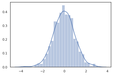
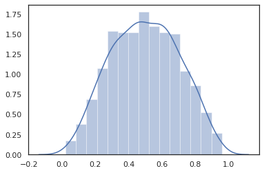
由于 JAX DeviceArray 与 NumPy 和 Matplotlib 等库兼容,我们可以直接将样本馈送给绘制函数。
sns.distplot(tfd.Normal(0., 1.).sample(1000, seed=random.PRNGKey(0)))
plt.show()
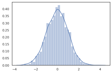
Distribution 方法与 JAX 转换兼容。
sns.distplot(jit(vmap(lambda key: tfd.Normal(0., 1.).sample(seed=key)))(
    random.split(random.PRNGKey(0), 2000)))
plt.show()
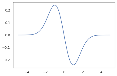
x = jnp.linspace(-5., 5., 100)
plt.plot(x, jit(vmap(grad(tfd.Normal(0., 1.).prob)))(x))
plt.show()
由于 TFP 分布作为 JAX pytree 节点注册,我们可以编写以分布作为输入或输出的函数,并使用 jit 对其进行转换,但还不支持将这些分布作为 vmap 函数的参数。
@jit
def random_distribution(key):
  loc_key, scale_key = random.split(key)
  loc, log_scale = random.normal(loc_key), random.normal(scale_key)
  return tfd.Normal(loc, jnp.exp(log_scale))
random_dist = random_distribution(random.PRNGKey(0))
print(random_dist.mean(), random_dist.variance())
0.14389051 0.081832744
转换的分布
转换的分布就是通过 Bijector 传递样本的分布,也是立即可供使用(双射函数也可用!请参阅下文)。
dist = tfd.TransformedDistribution(
    tfd.Normal(0., 1.),
    tfb.Sigmoid()
)
sns.distplot(dist.sample(1000, seed=random.PRNGKey(0)))
plt.show()
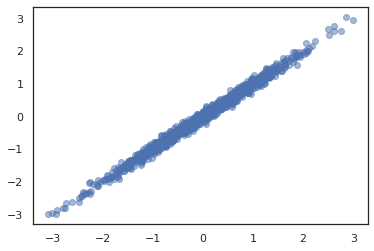
联合分布
TFP 提供了 JointDistribution,可用于将各个组件分布合并为多个随机变量的单一分布。目前,TFP 提供了三个核心变体(JointDistributionSequential、JointDistributionNamed 和 JointDistributionCoroutine),它们均可以在 JAX 中使用。另外,JAX 也支持 AutoBatched 的所有变体。
dist = tfd.JointDistributionSequential([
  tfd.Normal(0., 1.),
  lambda x: tfd.Normal(x, 1e-1)
])
plt.scatter(*dist.sample(1000, seed=random.PRNGKey(0)), alpha=0.5)
plt.show()
joint = tfd.JointDistributionNamed(dict(
    e=             tfd.Exponential(rate=1.),
    n=             tfd.Normal(loc=0., scale=2.),
    m=lambda n, e: tfd.Normal(loc=n, scale=e),
    x=lambda    m: tfd.Sample(tfd.Bernoulli(logits=m), 12),
))
joint.sample(seed=random.PRNGKey(0))
{'e': DeviceArray(3.376818, dtype=float32),
 'm': DeviceArray(2.5449684, dtype=float32),
 'n': DeviceArray(-0.6027825, dtype=float32),
 'x': DeviceArray([1, 1, 1, 1, 1, 1, 1, 1, 1, 1, 1, 1], dtype=int32)}
Root = tfd.JointDistributionCoroutine.Root
def model():
  e = yield Root(tfd.Exponential(rate=1.))
  n = yield Root(tfd.Normal(loc=0, scale=2.))
  m = yield tfd.Normal(loc=n, scale=e)
  x = yield tfd.Sample(tfd.Bernoulli(logits=m), 12)

joint = tfd.JointDistributionCoroutine(model)

joint.sample(seed=random.PRNGKey(0))
StructTuple(var0=DeviceArray(0.17315261, dtype=float32), var1=DeviceArray(-3.290489, dtype=float32), var2=DeviceArray(-3.1949058, dtype=float32), var3=DeviceArray([0, 0, 0, 0, 0, 0, 0, 0, 0, 0, 0, 0], dtype=int32))
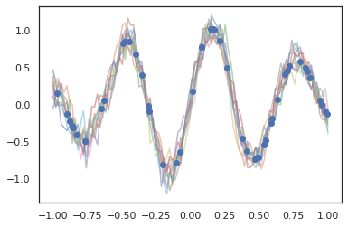
其他分布
高斯过程也可以在 JAX 模式下使用!
k1, k2, k3 = random.split(random.PRNGKey(0), 3)
observation_noise_variance = 0.01
f = lambda x: jnp.sin(10*x[..., 0]) * jnp.exp(-x[..., 0]**2)
observation_index_points = random.uniform(
    k1, [50], minval=-1.,maxval= 1.)[..., jnp.newaxis]
observations = f(observation_index_points) + tfd.Normal(
    loc=0., scale=jnp.sqrt(observation_noise_variance)).sample(seed=k2)

index_points = jnp.linspace(-1., 1., 100)[..., jnp.newaxis]

kernel = tfpk.ExponentiatedQuadratic(length_scale=0.1)

gprm = tfd.GaussianProcessRegressionModel(
    kernel=kernel,
    index_points=index_points,
    observation_index_points=observation_index_points,
    observations=observations,
    observation_noise_variance=observation_noise_variance)

samples = gprm.sample(10, seed=k3)
for i in range(10):
  plt.plot(index_points, samples[i], alpha=0.5)
plt.plot(observation_index_points, observations, marker='o', linestyle='')
plt.show()
JAX 也支持隐马尔可夫模型。
initial_distribution = tfd.Categorical(probs=[0.8, 0.2])
transition_distribution = tfd.Categorical(probs=[[0.7, 0.3],
                                                 [0.2, 0.8]])

observation_distribution = tfd.Normal(loc=[0., 15.], scale=[5., 10.])

model = tfd.HiddenMarkovModel(
    initial_distribution=initial_distribution,
    transition_distribution=transition_distribution,
    observation_distribution=observation_distribution,
    num_steps=7)

print(model.mean())
print(model.log_prob(jnp.zeros(7)))
print(model.sample(seed=random.PRNGKey(0)))
[3.       6.       7.5      8.249999 8.625001 8.812501 8.90625 ]
/usr/local/lib/python3.6/dist-packages/tensorflow_probability/substrates/jax/distributions/hidden_markov_model.py:483: UserWarning: HiddenMarkovModel.log_prob in TFP versions < 0.12.0 had a bug in which the transition model was applied prior to the initial step. This bug has been fixed. You may observe a slight change in behavior.
  'HiddenMarkovModel.log_prob in TFP versions < 0.12.0 had a bug '
-19.855635
[ 1.3641367  0.505798   1.3626463  3.6541772  2.272286  15.10309
 22.794212 ]
JAX 还不支持 PixelCNN 等少数几种分布,因为它们严重依赖于 TensorFlow 或者与 XLA 不兼容。
双射器
现在,JAX 支持 TFP 的大部分双射器!
tfb.Exp().inverse(1.)
DeviceArray(0., dtype=float32)
bij = tfb.Shift(1.)(tfb.Scale(3.))
print(bij.forward(jnp.ones(5)))
print(bij.inverse(jnp.ones(5)))
[4. 4. 4. 4. 4.]
[0. 0. 0. 0. 0.]
b = tfb.FillScaleTriL(diag_bijector=tfb.Exp(), diag_shift=None)
print(b.forward(x=[0., 0., 0.]))
print(b.inverse(y=[[1., 0], [.5, 2]]))
[[1. 0.]
 [0. 1.]]
[0.6931472 0.5       0.       ]
b = tfb.Chain([tfb.Exp(), tfb.Softplus()])
# or:
# b = tfb.Exp()(tfb.Softplus())
print(b.forward(-jnp.ones(5)))
[1.3678794 1.3678794 1.3678794 1.3678794 1.3678794]
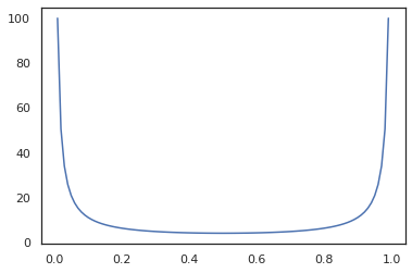
双射器与 jit、grad 和 vmap 等 JAX 转换兼容。
jit(vmap(tfb.Exp().inverse))(jnp.arange(4.))
DeviceArray([ -inf, 0. , 0.6931472, 1.0986123], dtype=float32)
x = jnp.linspace(0., 1., 100)
plt.plot(x, jit(grad(lambda x: vmap(tfb.Sigmoid().inverse)(x).sum()))(x))
plt.show()
不过,现在还不支持 RealNVP 和 FFJORD 等部分双射器。
MCMC
此外,我们还将 tfp.mcmc 移植到 JAX 中,因此,可以在 JAX 中运行汉密尔顿蒙特卡洛 (HMC) 和 No-U-Turn-Sampler (NUTS) 等算法。
target_log_prob = tfd.MultivariateNormalDiag(jnp.zeros(2), jnp.ones(2)).log_prob
与 TF 上的 TFP 不同的是,我们需要使用 seed 关键字参数将 PRNGKey 传递到 sample_chain 中。
def run_chain(key, state):
  kernel = tfp.mcmc.NoUTurnSampler(target_log_prob, 1e-1)
  return tfp.mcmc.sample_chain(1000,
      current_state=state,
      kernel=kernel,
      trace_fn=lambda _, results: results.target_log_prob,
      seed=key)
states, log_probs = jit(run_chain)(random.PRNGKey(0), jnp.zeros(2))
plt.figure()
plt.scatter(*states.T, alpha=0.5)
plt.figure()
plt.plot(log_probs)
plt.show()
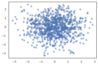
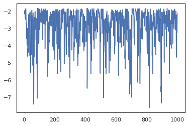
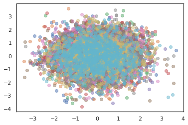
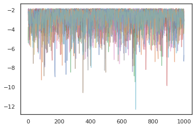
为了运行多个链,我们可以将一批状态传递到 sample_chain 中,也可以使用 vmap(不过我们尚未探索这两种方式在性能方面的差异)。
states, log_probs = jit(run_chain)(random.PRNGKey(0), jnp.zeros([10, 2]))
plt.figure()
for i in range(10):
  plt.scatter(*states[:, i].T, alpha=0.5)
plt.figure()
for i in range(10):
  plt.plot(log_probs[:, i], alpha=0.5)
plt.show()
优化器
JAX 上的 TFP 支持一些重要的优化器,例如 BFGS 和 L-BFGS。我们来设置一个简单的定标平方损失函数。
minimum = jnp.array([1.0, 1.0])  # The center of the quadratic bowl.
scales = jnp.array([2.0, 3.0])  # The scales along the two axes.

# The objective function and the gradient.
def quadratic_loss(x):
  return jnp.sum(scales * jnp.square(x - minimum))

start = jnp.array([0.6, 0.8])  # Starting point for the search.
BFGS 可以找到此损失的最小值。
optim_results = tfp.optimizer.bfgs_minimize(
    value_and_grad(quadratic_loss), initial_position=start, tolerance=1e-8)

# Check that the search converged
assert(optim_results.converged)
# Check that the argmin is close to the actual value.
np.testing.assert_allclose(optim_results.position, minimum)
# Print out the total number of function evaluations it took. Should be 5.
print("Function evaluations: %d" % optim_results.num_objective_evaluations)
Function evaluations: 5
L-BFGS 也可以找到此损失的最小值。
optim_results = tfp.optimizer.lbfgs_minimize(
    value_and_grad(quadratic_loss), initial_position=start, tolerance=1e-8)

# Check that the search converged
assert(optim_results.converged)
# Check that the argmin is close to the actual value.
np.testing.assert_allclose(optim_results.position, minimum)
# Print out the total number of function evaluations it took. Should be 5.
print("Function evaluations: %d" % optim_results.num_objective_evaluations)
Function evaluations: 5
为了对 L-BFGS 执行 vmap,我们设置一个函数,用于优化单一起始点的损失。
def optimize_single(start):
  return tfp.optimizer.lbfgs_minimize(
      value_and_grad(quadratic_loss), initial_position=start, tolerance=1e-8)

all_results = jit(vmap(optimize_single))(
    random.normal(random.PRNGKey(0), (10, 2)))
assert all(all_results.converged)
for i in range(10):
  np.testing.assert_allclose(optim_results.position[i], minimum)
print("Function evaluations: %s" % all_results.num_objective_evaluations)
Function evaluations: [6 6 9 6 6 8 6 8 5 9]
注意事项
TF 与 JAX 之间存在一些根本区别,有些 TFP 行为在这两种基质之间有所不同,并不是所有功能均受支持。例如,
- JAX 上的 TFP 不支持任何诸如
tf.Variable一类的功能,因为此类功能在 JAX 中不存在。这也意味着tfp.util.TransformedVariable等实用工具也不受支持。 - 后端现在还不支持
tfp.layers,因为它依赖于 Keras 和tf.Variable。 tfp.math.minimize不适用于 JAX 上的 TFP,因为它依赖于tf.Variable。- 对于 JAX 上的 TFP,张量形状始终为具体的整数值,从来都是已知值,不像在 TF 上的 TFP 那样会动态变化。
- 在 TF 与 JAX 中,伪随机性的处理方式不同(请参阅附录)。
- 无法确保
tfp.experimental中的库也存在于 JAX 基质中。 - 数据类型提升规则在 TF 与 JAX 之间有所不同。为了保持一致,JAX 上的 TFP 尝试在内部遵守 TF 的数据类型语义。
- 双射器尚未注册为 JAX pytree。
要想查看可以在 JAX 上的 TFP 中使用的全部功能,请参阅 API 文档。
结论
我们已将众多 TFP 功能移植到 JAX 中,看到所有人构建的内容,我们感到非常激动。某些功能目前还不能使用;如果我们遗漏了对您来说很重要的内容(或者您发现了错误!),请跟我们联系。您可以发送电子邮件至 tfprobability@tensorflow.org,也可以在我们的 Github 仓库上提交议题。
附录:JAX 中的伪随机性
JAX 的伪随机数生成 (PRNG) 模型无状态。有状态模型的全局状态在每次随机绘制后都会发生变化,与有状态模型不同的是,该模型没有可变的全局状态。在 JAX 模型中,我们从 PRNG 密钥开始,该密钥类似于一对 32 位整数。我们可以使用 jax.random.PRNGKey 来构造这些密钥。
key = random.PRNGKey(0)  # Creates a key with value [0, 0]
print(key)
[0 0]
JAX 中的随机函数使用密钥确切地生成随机变量,也就是说,这些变量不应当重复使用。例如,我们可以使用 key 对正态分布值抽样,但我们不应当在其他位置再使用 key。此外,如果将同一个值传递给 random.normal,也会得到相同的值。
print(random.normal(key))
-0.20584226
那么,我们如何基于一个密钥绘制多个样本?答案就是密钥拆分。基本思路是,我们可以将一个 PRNGKey 拆分为多个密钥,并将每一个新密钥视为一个独立的随机源。
key1, key2 = random.split(key, num=2)
print(key1, key2)
[4146024105 967050713] [2718843009 1272950319]
密钥拆分是确定的,但没有顺序,因此,每个新密钥现在均可用于绘制一个不同的随机样本。
print(random.normal(key1), random.normal(key2))
0.14389051 -1.2515389
有关 JAX 确定性密钥拆分模型的更多详细信息,请参阅本指南。